Bayesian Analysis of Stochastic and Deterministic Processes in The Error Correction Model.
Rodney W. Strachan1, University of Liverpool Brett Inder, Monash University
ABSTRACT
In this article a method for joint estimation of the number of stochastic trends and the deterministic processes in a multivariate error correction model is presented. This approach takes advantage of the Laplace method of approximating integrals and, the second important contribution of the paper, careful elicitation of the prior for the cointegrating vectors from a prior on the cointegrating space. The approach follows the classical approaches of James (1969), Anderson (1951) and Johansen (1988 and 1991) and performs well when used to estimate the number of stochastic trends compared with information criteria in …nite samples in Monte Carlo experiments.
JEL classi…cation: C11; C32.
Keywords: Stochastic trend; Deterministic trend; Posterior probability; Grassman manifold; Stiefel manifold.
1Correspondoing author: Rodney W. Strachan, Department of Economics and Accounting, Uni-versity of Liverpool, Liverpool, L69 7ZH, Great Britain. Ph: +44 (0)151 794 3043, Fx: +44 (0)151 794 3028, email: [email protected]
1 Introduction.
Since its development by Granger (1983) and Engle and Granger (1987), the con-cept of cointegration has proven a valuable tool in economic analysis and has found applications in many theories such as for real business cycle models, term structure of interest rates, purchasing power parity, and money demand to name just a few. An important consideration in cointegration is the accurate determination, or esti-mation, of the number of stationary combinations,r: Many classical tests have been
developed for this purpose, although relatively few Bayesian tests exist. In an early study, Geweke (1996) proposed the use of predictive probabilities estimated using a Markov Chain Monte Carlo (MCMC) method to determine the rank. Other work by Kleibergen and Paap (forthcoming) also used an MCMC approach but produced a posterior distribution for the rank. While there have been a few other approaches (see for example Strachan, forthcoming), none of these has produced a simple, e¢cient test which performs consistently well.
The …rst aim of this paper is to present a simple Bayesian test for the rank which is related to the classical trace test developed by Anderson (1951) for the general reduced rank regression model and applied to the cointegrating ECM by Johansen (1988 and 1991). This test has similar performance to the trace test when used to estimate the number of stochastic trends, which is not surprising as it can be shown to be a simple function of the trace statistic for particular common priors.
In applied analysis, economic time series are commonly modelled as combinations of both stochastic and deterministic trends. Deterministic processes have implications for both theoretical and applied analysis of time series as evidenced by the range of distributions necessary to conduct classical inference in cointegrated models, the presence (or absence) of various deterministic processes a¤ects inference about the number of stochastic trends. This in‡uence is re‡ected in the changing location of the posterior distribution of r for models with di¤erent deterministic processes.
Therefore, we extend the analysis to consideration of various models of deterministic terms within the ECM and present a method for estimation of the joint posterior distribution of (r; i), where i is an indicator of the deterministic process present in
the model.
Important advantages of the Bayesian approach over the classical approach are the treatment of model uncertainty and greater ‡exibility to explicitly incorporate prior beliefs. Classical methods such as hypothesis tests on parameter values or the use of information criteria for model selection, result in subsequent inference being conditional upon the chosen model, regardless of the information content of ‘nearby’ models. Bayesian posterior probabilities, however, allow inference to be averaged over a range of models if the econometrician so desires.
The outline of the article is as follows. In Section Two the models are described. The likelihood, the priors and a general form for the posterior are given in Section
Three. An important contribution of this section, and indeed this paper, is the careful elicitation of the prior distribution on the cointegrating coe¢cients from a prior on the cointegrating space. An outline of the identifying restrictions which arise naturally from the prior elicitation is also provided. Section Four introduces the inferential tool, the Bayes factor and the application of Laplace approximation is presented in Section Five. Monte Carlo experiments are reported in Section Six and the technique is applied to an actual data set in Section Seven. Section Eight concludes.
Throughout this paper the notation ‘a ´ b’ implies that models a and b are
equivalent. The space spanned by a matrix A is denoted sp(A) and its jth largest
eigenvalue is ¸j(A), Vr;n = fV (n£r) :V0V =Irg is the Stiefel manifold, O(r) = fC(r£r) :C0C= Irg denotes the orthogonal group of r £r orthogonal matrices.
p 2 Gr;n¡r denotes that p is an r¡dimensional plane in n¡space, passing through the origin of that space, and hence pis an element of a Grassman manifold, Gr;n¡r: Importantly, for any V 2 Vr;n; there exists a plane p =sp(V)such that p2 Gr;n¡r: The reader is referred to Muirehead (1982) and in particular James (1954) for more details on these matrix spaces.
2 The model.
The error correction model (ECM) of the 1 £ n vector time series process yt =
(y1t; : : : ynt); t= 1; : : : ; T;conditioning on the l observationst=¡l+ 1; : : : ;0;is
¢yt = yt¡1¯+®+dt¹+ ¢yt¡1¡1+: : :+ ¢yt¡l¡l+"t (1)
= yt¡1¯+®+dt¹1®+dt¹2®?+ ¢yt¡1¡1+: : :+ ¢yt¡l¡l+"t
= z1;t¯®+z2;t© +"t (2)
where¢yt=yt¡yt¡1; z1;t = (dt; yt¡1); z2;t = (dt;¢yt¡1; : : : ;¢yt¡l);© = (®?0 ¹02;¡01; : : : ;¡0l)0 and ¯ =¡¹0; ¯+0¢0. The matrices¯+ and®0 aren£r and assumed to have rank r:
Of interest when considering the number of stochastic trends is the coe¢cient matrix ¯ which is of dimension ni £r; where ni depends upon the deterministic processes present and is de…ned in the next section, and rank(¯®) = r ·n. When
r < n this impliesyt is cointegrated. Expressing z1;t¯ as z1;t¯ =dt¹1+yt¡1¯+; then
¯+ is the matrix of cointegration coe¢cients and ® is the matrix of factor loading
coe¢cients or adjustment coe¢cients.
The (j+ 1)th element of the vectordt;istj such thatdtcontains the deterministic terms such as constants and trends. We will restrict ourselves to consideringj 2(0;1)
such that dt = (1; t) and ¹ = (a ±)0 = ¹1®+¹2®?: Restricitions on these trends and constants entering either the levels, yt; or the cointegrating relations, yt¯+; are discussed further in the next subsection.
Finally, introduce the following terms to simplify the expressions in the posteriors. Let ezt = (z1;t¯ z2;t); and the(r+ki)£nmatrix B = [®0 ©0]0:The model may now be written as
¢yt= eztB+": (3)
2.1 Deterministic terms
It is well known that simplistic treatment of the deterministic terms by testing whether
¹or some elements of¹are zero leads to the strange and unsatisfactory situation that
very di¤erent trending behaviour is implied in the levels of the process for di¤ering values of r: For example, a nonzero intercept, a, in (1) simply produces a nonzero
mean when r =n, but it could induce a linear drift in yt and a nonzero mean for the error correction term,yt¯+;whenr < n. It is for the purpose of incorporating a range of deterministic behaviours, such as drifts and trends in the cointegrating relations and in the levels, that¹ is decomposed into ¹=¹1®+¹2®? where ¹1= ¹®0(®®0)¡
1
and ¹2=¹®0?(®?®0?)¡
1 (see Johansen, 1995 Section 5.7 for further discussion). Economists are commonly interested in the presence or absence of deterministic processes in yt oryt¯+: Important are questions such as whether linear or quadratic drifts are present inyt and whether nonzero constant terms and deterministic trends are present in yt¯+: Assuming dt = (1; t);then for each j = 1;2; dt¹j =¹j;¶+t¹j;±: Although a wider range of models are clearly available, the …ve most commonly
considered may be stated as follows, where Mr;i is the ith model of deterministic terms at given rankr :
Mr;1 : dt¹=¹1;¶®+¹2;¶®?+¡¹1;±®+¹2;±®?¢t
Mr;2 : dt¹=¹1;¶®+¹2;¶®?+¹1;±®t
Mr;3 : dt¹=¹1;¶®+¹2;¶®?
Mr;4 : dt¹=¹1;¶®
Mr;5 : dt¹= 0
A total of 5 (n+ 1) models of deterministic terms and numbers of stochastic terms
are considered in this article. Notice that at r = n, Mn;1 ´ Mn;2 and Mn;3 ´ Mn;4 since ®? = 0. Similarly, atr = 0; M0;2´ M0;3and M0;4´M0;5 since® = 0. Finally,
ni =n+ 2 fori= 1;2; ni =n+ 1fori = 3;4and ni=n fori= 5:
3 Priors and posteriors.
In this section the forms of the priors and resultant posterior are presented. We restrict ourselves to ‡at priors where possible, although consideration is given to informative priors when discussing the parameters of interest. For the model in (3), assume the rows of " = ("0
1; "02; : : : ; "0T)0 are"t s iidN(0;§):The likelihood can then be written asL³yj§; B; ¯; r;Ze´/ j§j¡T2 exp©¡1
2tr(§¡1"0")
ª
3.1 The prior for (§; B; r; i):
Throughout this paper, the prior for the rankr isp(r) = (n+ 1)¡1and for the deter-ministic models p(i) = 1=5. The standard di¤use prior for §; p(§)_ j§j¡(n+1)=2; is
used.
The matrix B changes dimensions across the di¤erent models Mr;i: Thus if the prior on B is p(Bj¯; r; i) = cr;ih(B) where c¡r;i1 =
R
h(B) (dB); then clearly cr;i depends upon(r; i):As discussed in O’Hagan (1995), Bayes factors forMr;i toMr¤;i¤;
from which the posterior probabilities are derived, are proportional to the ratio¶ =
cr;i=cr¤;i¤ and therefore knowledge of¶ is required. If an improper prior on B such as
h(B) = 1, were used, then cr;i does not exist but can be treated as an unspeci…ed constant such that cr;i=cr;i = 1 and as a result the posterior will be well de…ned. However, as ¶ will be unspeci…ed, the resulting Bayes factors can not be obtained. For this reason a (weakly) informative proper prior forB must be used. In this article,
the prior for B conditional upon(§; ¯; r; i) is normal with zero mean and covariance §-³¯e0He¯´¡1whereH = 0:01I(n+ki) and e ¯ = 2 6 6 4 ¯ 0 0 Iki 3 7 7 5:
3.2 Eliciting a prior on ¯:
Linear restrictions and the cointegrating space: It is well known that as¯ and
® appear as a product in (2), r2 restrictions need to be imposed on the elements of ¯
and ®to just identify these elements. These restrictions are commonly imposed upon ¯by assumingc¯is invertible for known matrixcand the restricted¯is¯ =¯(c¯)¡1:
Thus the free elements are collected in ¯2 =c?¯wherec?c0 = 0:A common choice in theoretical work isc= [Ir 0]such that¯ = [Ir ¯02]0: A prior is then speci…ed for¯2:
The practical problems in classical analysis of incorrectly selectingcwere discussed
in Boswijk (1996) and Luukkonen, Ripatti and Saikkonen (1999) and in Bayesian analysis by Strachan (forthcoming). In each of these papers compelling examples were provided of the importance of correctly determining c: Assumng known c; the
pathologies and complicating features (for analysis) of the posterior for ¯2with a ‡at prior, such as multimodality, nonexistence of moments and (under some speci…cations) impropriety of the posterior have been detailed by Kleibergen and van Dijk (1994) and Bauwens and Lubrano (1996). In addition, unpublished notes by Bauwens and Lubrano showed nonexistence of the posterior when another important and commonly employed restriction on (2), exogeneity, is imposed. Further, from the discussion on the prior for B it is clear a ‡at prior on¯2 cannot be employed to obtain posterior probabilities for(r; i); since the dimensions of¯2 depend upon(r; i):
to explicitly incorporate prior beliefs into the analysis. As a ‡at prior is generally intended to re‡ect ignorance about the parameter of interest, the above issues with the posterior at least, may be resolved by use of an informative prior on ¯2:However, to preserve the options of both informative and uninformative priors, as the issue of selectingcis not resolved by a proper prior, and as we do not see¯2as the parameter of interest, we therefore diverge at this point from much of the earlier literature (except Villani 2000) in both specifying our parameter of interest and eliciting uninformative and informative priors on that parameter.
In cointegration analysis it is not the values of the elements of ¯ that are the
object of interest, rather the space spanned by ¯; p = sp(¯); and this space is in
fact all we are able to uniquely estimate. The parameter pis an r¡plane inn¡space (ignoring for now the dependence onni and assumeni =n) and as such an element of the Grassman manifold Gr;n¡r : Before we derive the priors forp we brie‡y comment on the relationship between priors on ¯2 and on p:
The Jacobian for the transformation fromp2 Gr;n¡r to¯2 2R(n¡r)r is presented in Villani (2000) as jIr+¯02¯2j¡
n=2
:Although Villani (2000) usesc= [Ir 0];this form holds for generalcand is the kernal of a Cauchy density. From this Jacobian we can
clearly see that a ‡at prior onpis informative with respect to¯2and vice versa. This result re‡ects that found by Phillips (1994) in classical analysis when an element of the Steifel manifold - which de…nes an element of a Grassman manifold - is renormalised
by imposing linear restrictions. That is Phillips (1994) shows that the …nite sample distribution of the maximum likelihood estimator with linear restrictions imposed has Cauchy tails and that this Cauchy behaviour is a direct result of imposing the linear restrictions.
Next consider the implications of a ‡at prior on ¯2 for the prior onp. A common
justi…cation for the linear restrictions is that an economist will usually have some idea about which variables will enter the cointegrating relations and so she choosesc
to select the rows of coe¢cients most likely to be nonzero - more generally linearly independent from eachother - and then normalise on these coe¢cients. This is a necessary assumption to ensure (c¯)¡1 exists. By using these linear restrictions,
however, the Jacobian for ¯2 ! p places more weight in the direction where the coe¢cients thought most likely to be di¤erent from zero are, in fact, zero (or linearly dependent).
To demonstrate this claim, consider an¡dimensional system fory = (x0; z0)0where xis arvector. To use linear restrictions a normalisation must be chosen by choice ofc.
It is believed that if a cointegrating relationship exists then it will most likely involve the elements ofxin linearly independent relations:That is in y¯ =x¯1+z¯2 vI(0), det (¯1) is believed far from zero making it safe to normalise on ¯1; and so choose
transformation ¯2!p is proportional to
J(¯2:¯) = ¯¯Ir+ (c¯)0¡1¯0c0?c?¯(c¯)¡1¯¯ n=2
:
Asp=sp(¯)!sp(c); c?¯ !0(n¡r)£randc¯ ! O(r)andJ(¯2:¯)! 1. However, as vectors in¯ approach the null space of c, that is det (c¯) !0; then(c¯)¡1! 1;
and thus J(¯2 :¯) ! 1. As a result the prior will more heavily weight regions
wheredet (c¯) = det (¯1)t0;contrary to the intention of the economist. As a trivial
example, if r = 1; we would choose c = (1;0; : : : ;0) as we believe ¯1 6= 0: Yet the Jacobian places in…nite weight in the region of¯1= 0:
A uniform prior on the cointegrating space: Clearly then there is reason to consider another approach to eliciting priors for ¯. Our recommendation is, if the
economist wishes to incorporate prior beliefs about the cointegrating relations, these should be expressed in the prior distribution for the cointegrating space.
As we have claimed the cointegrating space to be the parameter of interest, we propose working directly withp=sp(¯) and avoiding the linear restrictions. Initially a distribution and identifying restrictions for ¯ from the uniform distribution for p
overGr;n¡r is derived using the results of James (1954). This prior has the form
p(¯) (¯0d¯) = R 1 (¯0d¯)(¯
0d¯)
where (¯0d¯) is the exterior product di¤erential form for the free elements of ¯ and de…nes the invariant (to left and right orthogonal translations) measure onGr;n¡rand
is equivalent to the product of the Jacobian for the transformation from p to¯ and
the di¤erential for the elements of ¯ (see James 1954, Muirhead 1982, Ch. 2). This
expression for the prior de…nes a probability measure on the space of ¯: Throughout
the paper, to save on notation we omit the di¤erential term for all parameters except
¯ as this is the focus of the analytical results.
As the support of ¯ is a function of (r; i); so will be R (¯0d¯)2: Therefore to
employ the above distribution it is necessary to …nd the explicit form for R (¯0d¯):
This is obtained by using the relationship between Gr;n¡r and the Steifel manifold and orthogonal group. We reproduce this result from James (1954) as we will rely on some of its implications later. If A 2 Vr;ni and p= sp(A); then p2 Gr;ni¡r and
A is determined uniquely given p and orientation of A in p byC 2O(r), such that
A=¯C where¯ 2Vr;ni; sp(¯) =p: James (1954)3 shows
Z Gr;ni¡r (¯0d¯) = R Vr;ni(A0dA) R O(r)(C0dC) (4) = ¼¡(ni¡r)r¦rj=1 ¡ [(ni+ 1¡j)=2] ¡ [(r+ 1¡j)=2] where ¡ [q] =R01uq¡1e¡udu q >0:
In early work in this area, Villani (2000) also began with a uniform prior upon the cointegrating space from which he derived the prior distribution for ¯2: However
2The authors are grateful to an anonymous referee for pointing out the importance of this de-pendence in development of the posterior.
his interest was in estimation and tests related tosp(¯) and as such, the analysis was
conditional upon (r; i). For reasons discussed earlier, we wish to avoid using linear
restrictions to identify ¯ and thus must …nd an alternative set of restrictions that do
not require knowledge ofcand which avoid the issues associated with the posterior for ¯2:Fortunately the de…nition ofAprovides a natural solution to this question. That is use¯ 2Vr;ni which impliesr(r+ 1)=2restrictions, with the usual assumption about …xing the sign of the element in the …rst row. This latter assumption simply restricts the vectors of ¯ to one half hemisphere but in no way restricts the estimable space.
Although the dimension of the Grassman manifold is only (ni¡r)r; the remaining
r(r¡1)=2 restrictions come from the orientation by C. The prior, the posterior (as
is made clear later) and the di¤erential form for ¯ are all invariant to translations of the form ¯ ! ¯H; H 2 O(r): Therefore it is possible to work directly with ¯
as an element of the Steifel manifold and adjust the integrals with respect to ¯ by
³R
O(r)(C0dC)
´¡1
as shown in (4). Note that these identifying restrictions do not distort the weight on the space of the parameter of interest,p.
An informative prior on the cointegrating space: Although the uniform prior (4) is used in this paper, it is common to employ informative priors for parame-ters and so one is speci…ed here for p.
If an economist believes a parameter is likely to have a particular value, to incor-porate this prior belief she places more prior mass around this likely point. For the
parameter p, we will denote the likely value as pH =sp(H·) where H 2 V
s;n (again we ignore the dependence onni and assume ni =n) is a knownn£s (s¸ r)matrix,
H?2Vn¡s;n its orthogonal compliment and·is ans£rfull rankr matrix. To obtain
H; specify the general matrix Hg with the desired coe¢cient values, then map this toVr;n by the transformation H=Hg(Hg0Hg)¡1=2:
A dogmatic prior forp could be obtained by letting ¯= H·V; V 2O(r):De…ne ·V =V·2 Vr;s and specify the prior in (4) for V·: This prior assigns probability one to the point p= pH:
Often, however, the economist will want to employ a less dogmatic prior such that there is some weight away from the likely value. A possible speci…cation for this prior follows. Let the random scalar ¿ have E(¿) = 0 and E(¿2) =¾2:The value of ¾ will control the tightness of the prior around pH. Next construct
P¿ = HH0+H?H?0¿ = [H H?] 2 6 6 4 Ir 0 0 In¡r¿ 3 7 7 5 2 6 6 4 H0 H?0 3 7 7 5
and let the elements of then£r matrixZ be independently distributed as standard normal,N(0;1):The matrixX =P¿Z can be decomposed asX =¯· where¯ 2Vr;n and · is an r£r lower triangular matrix. For ¿ = 06 and j¿j <1; the space of ¯;
p = sp(¯); is a direct weighted sum of the spaces pH and pH? with the weight
At ¿ = 0 and ¿ = §1; p is respectively pH and pH?. It is for this reason that we choseE(¿) = 0 such that with respect to¿, the space will on average bepH: One choice for ¿ is N(0;1). Integrating with respect to K =··0 which is distributed as
Wishart, the form of the resultant prior for ¯ and the hyperparameter ¿ is p(¿; ¯) (¯0d¯) (d¿) =¿¡(ni¡r)rexp ½ ¡¿ 2 2 ¾ ¯¯ ¯0P¿¡21¯¯¯ ¡n=2 c(r;i)(¯0d¯) (d¿)
where c(r;i) = 2¡r¡1=2¼r(r¡1)=4¡(n+1)r=2¦rj=1¡ [(ni+ 1¡j)=2]: This prior treats the area around pH?; which occurs at ¿ = 1; as an extreme (practically impossible)
event regardless of the choice of ¾. This is desirable since at ¿ =1 the dimension of the cointegrating space, dim (p); would become dim¡pH?¢ = min (p¡r; r) rather than r:
As an alternative, if the researcher would prefer to assign more weight in the direction of pH? but preserve dim (p) = r with probability one, she may choose
P¿ = HH0(1¡¿2)1=2+ H?H?0¿ with ¿ 2 [¡1;1]: Again the choice of E(¿) = 0 would make sense and E(¿2) = ¾2 controls the tightness of the prior around pH. A possible choice of a distribution for´=¿+ 1may be Beta over ´2[0;2]which allows
some mass to be distributed around pH? by appropriate choice of parameter values.
An MC(MC) scheme for obtaining draws from the posterior with either the uni-form or inuni-formative prior could be developed using the uni-form of the above inuni-formative prior as a candidate density in which H is set near to the mode of the posterior (see Appendix). Draws of ¯ could then be drawn using the above outline by drawing ¿
and Z; then constructingX then¯; giving a draw of (¿; ¯). Finally, the value of ¾
could be calibrated to a preferred level of dispersion using the span variation measure (sv) of Larsson and Villani (2001), developed further in Villani (2000), and MC(MC)
draws. Villani (2000) shows how sv can be used to express the degree of variation
in a distribution for as a proportion of the variation under the uniform distribution -the uniform providing equal variation in every direction.
3.3 The posteriors.
Using the priors speci…ed above, the general form of the posterior is then
p(B;§; ¯; r; ijy) / j§j¡(T+n+r+ki+1)=2 £exp ½ ¡1 2tr§ ¡1 · T S+³B¡Be´0V ³B¡Be´¸¾ (5) £(2¼)¡n(ki+r)=2100¡n(ki+r)=2p(¯) (¯0d¯) where S = S00¡S01¯(¯0S11¯)¡1¯0S10; Be = · e ®0 ©e0 ¸0 , ®e = (¯0S11¯)¡1¯0S10; © =e S¡221S20;andV =e¯ 0¡ §T
t=1zt0zt+H¢ e¯ where zt= (z1;t z2;t). The values for theSij are de…ned as
ºMij = hij+ §Tt=1zi;t0 zj;t fori and j = 1;2;
hij = 0 if i6=j andhii= 0:01I;
ºM20 = §Tt=1z02;t¢yt; ºM10= §Tt=1z01;t¢yt;
excepti=j = 2 where
S22 =M22¡M21M11¡1M12 and S20 =M20¡M21M11¡1M10: For later use we also de…ne D0=D1¡D2; D1=S11 and D2= S01S11¡1S10:
4 Bayes factors and posterior probabilities.
In this section the tool for Bayesian inference in this paper - the posterior probabilities of the ranks - is introduced. Our objective is to report estimates of the posterior probabilities of the modelMi;r; p(Mi;rjy) = p(i; rjy):LetBkl be the Bayes factor for the model Mk; k = (r; i) to the model Ml, l = (r¤; i¤). The posterior probabilities and the Bayes factors are linked through the expression for the posterior odds ratio. First consider the posterior odds ratio for model Mk to modelMl with parametersµk and µl respectively, p(kjy) p(ljy) = p(k)R L(µk)p(µkjk)d(µk) p(l)R L(µl)p(µljl)d(µl) = p(k) p(l) £ m(yjk) m(yjl) = p(k) p(l) £Bk;l:
where p(k)is the prior probability of the model k and
m(yjk) =
Z
L(µk)p(µkjk)d(µk) (6) is the marginal likelihood for the modelk. As the prior odds are known, we need only estimate Bk;l.
To estimate the relevant Bayes factors for the models of interest, estimates of the marginal likelihoods in (6) are required. To perform the integration in (6) of µk =
(§; B; ¯); …rst analytically integrate (5) with respect to(§; B):From the expression
in (5), it is straight forward to show that the posterior for (§; B) conditional on (¯; r; i) has a standard form which may be integrated analytically (see for example Zellner, 1971). The resulting posterior for the remaining parameters is
p(¯; r; ijy)_g(r;i)jS00j¡T =2jM22j¡n=2j¯0D0¯j¡T =2j¯0D1¯j(T¡n)=2(¯0d¯) (7) where in this case g(r;i) =T¡nr=2¼¡(ni¡r)r=2100¡n(ki+r)=2: The conditional density for
¯ given (r; i) has the form
p(¯jr; i; y) (¯0d¯) _ j¯0D0¯j¡T=2j¯0D1¯j(T¡n)=2(¯0d¯)
= k(¯) (¯0d¯)
wherek(¯) =j¯0D0¯j¡T =2j¯0D1¯j(T¡n)=2:(¯0d¯)is invariant to¯!¯CforC 2O(r) and the above form makes it clear that so isk(¯):The eigenvalues¸j(Dl)forl = 0;1; will be positive and …nite with probability one. By the Poincaré separation theorem, since¯2Vr;n; then¦rj=1¸n¡r+j(Dl)· j¯0Dl¯j ·¦rj=1¸j(Dl)and so k(¯)is bounded above (and below) by some positive …nite constant. Also, (¯0d¯) is integrable and
therefore …nite almost everywhere. Thus k(¯) (¯0d¯) has a …nite upper bound,M.
As the elements of ¯; bij;have compact support, the integral
R
Vr;nb m
ijk(¯) (¯0d¯) for will be bounded above almost everywhere by the integral R1 m .
These conditions are su¢cient to ensure the posterior for ¯ will be proper and all
…nite moments exist (see Billingsley 1979, pp. 174 and 180).
To obtain the posterior distribution of (r; i); p(r; ijy); it is necessary to integrate
(7) with respect to ¯ and so obtain an expression for p(r; ijy) = Z p(¯; r; ijy)d¯ = Z p(¯jr; i; y)p(r; ijy)d¯ = Z p(¯jr; i; y)d¯p(r; ijy): (8)
The marginal density of ¯ conditional on r has the same form in all cases as p(¯jr; i; y) =c(r;i)¡1 k(¯) (¯0d¯) (9) which is not of standard form. Although one may exist, we do not currently know of a simple, general analytical solution for c(r;i) =
R
Vr;nk(¯) (¯0d¯) and so we estimate
c(r;i).
Two possible approaches to estimatingc(r;i) are either to use Markov Chain Monte Carlo (MCMC) methods or numerical integration. Kleibergen and Paap (forthcom-ing) and Bauwens and Lubrano (1996) demonstrate how to evaluate similar integrals using MCMC when ¯ has been identi…ed using linear restrictions rather than those
used in this paper. Strachan (forthcoming) demonstrates the MCMC approach when
¯ has been identi…ed using related restrictions, how ever the posterior has a very di¤erent form as an embedding approach similar to Kleibergen and Paap is used. An
alternative approach commonly used in classical work to approximate integrals over
Vr;n;is to use the Laplace approximation which is computationally much faster. In the following section the Laplace approximation to a general integral is brie‡y outlined and applied to obtain an estimate of c(r;i):
5 Laplace approximation.
Letµ be am-dimensional vector of parameters. Iflnf= lnf(µ)is a smooth, positive
function with a maximum at µ; then by the Laplace method the integral R gf·dµ
can be approximated by g¡µ¢f·¡µ¢ ¡2¼ ·
¢m
2 jªj¡12 where ª is the Hessian of ¡lnf,
evaluated atµ =µ (g= g(µ)is a continuous nonzero function aroundµ). There are a
number of papers on applications of the Laplace approximation in econometrics (see for example Lindley 1980, Tierney & Kadane 1986, Tierney, Kass & Kadane 1989, Kass & Raftery 1995). However for more relevant references for our application to an integral over the Stiefel manifold the reader is directed to Muirehead (1982, Ch. 9), G.A. Anderson (1965) and James (1969). In these applications the aim was to derive distributions of latent roots of covariance matricies and the Laplace approach was used to provide asymptotic representations of hypergeometric functions of zonal polynomials which can be represented as integrals over the orthogonal group or, in some cases, the Stiefel manifold.
and if the posterior is reasonably peaked around the mode (Tierney and Kadane 1986, Tierney, Kass & Kadane 1989, Kass and Raftery 1995). Expressions for the mode and Hessian are presented in the Appendix. The posterior tends to be peaked for reasonable sample sizes and the mode dominates asT increases. On the general
ques-tion of approximating the marginal likelihood, c(r;i), by the Laplace approximation,
there is considerable precedent in the literature for using this method for this purpose (Lindley 1980, Kass & Vaidyanathan 1992, Raftery 1994, Kass & Raftery 1995, Lewis & Raftery 1997). Further, the results presented in this paper support the application of Laplace approximation at least for estimation of r.
To apply the Laplace approximation, let k = fTg; µ = ¯, m = r2(2ni¡r¡1);
· =T ; f =j¯0D0¯j¡1=2j¯0D1¯j1=2 andg =j¯0D1¯j¡n=2: The value of ¯ at the mode of f will be denoted as ¯ and the Hessian matrix for rank r evaluated at ¯ will
be ª = ªr: Johansen (1991) presents a modal estimator for f(¯); b¯; from which we could obtain ¯ = b¯³¯b0b¯´¡1=2 2 Vr;n. However, a slightly di¤erent derivation is
presented in the Appendix such that¯ =D1=21 b¯so¯ is ther eigenvectors associated with the eigenvalues ¸i
³
D¡11=2D2D¡11=2
´
for i = 1; : : : ; r: This approach simpli…es derivation of the Hessian which is also presented in the Appendix.
Using (7), (8), and (9), approximate p(r; ijy)by
b p(r; ijy) = µ2¼ T ¶r(2ni¡r¡1)=2 g¡¯¢f·¡¯¢jªrj¡12
The classical maximum eigenvalue test statistic, which is a likelihood ratio test statistic for the hypothesis H0 :rank(¦) = r versus H1 :rank(¦) = r + 1; has the form mr;r+1= ¡T ln
³
1¡b¸r+1
´
: From this expression it is possible to show the link
between the classical test statistic, mr;r+1; and the Bayes factor, B(r;i)(r+1;i), for the di¤use prior asBb(r;i)(r+1;i) =crexp (¡0:5mr;r+1)where cr depends on the data,r;and
n: Denote the classical trace test statistic, which is a likelihood ratio test statistic
for the hypothesis H0 : rank(¦) = r versus H1 : rank(¦) = n; as mr;n: Similarly, it is possible to present the link between mr;n and the Bayes factor, B(r;i)(n;i), for the di¤use prior asBb(r;i)(n;i)= ¦nj=rcjexp (¡0:5mr;n):
6 Monte Carlo experiment.
To investigate the small sample performance of our estimator forp(r; ijy), we conduct Monte Carlo experiments and compare these results to those for the a range of infor-mation criteria and the classical trace test. In the next section, the test is applied to a set of real data.
The general DGP for the experiments is a VAR with 2 lags and deterministic processes ¹jt = ¹j +±jt for j = 0;1;2: Let ¯2 be a (n¡r) £ r matrix, w1;t be a 1 £ r random vector and w2;t be a 1 £ (n¡r) random vector is generated by
wj;t = ¹jt +wj;t¡1½j +"j;t; j = 1;2 where "j;t v iidN(0; ¾2) and ½j is an identity matrix times ½: The 1£n vector of variables in the system is yt = (y1;t y2;t) where
y1;t is a 1£r random vector andy2;tis a1£(n¡r)random vector jointly generated by y1;t =¹0t+y2;t¯2+w1;t; y2;t=y2;t¡1+w2;t.
This speci…cation corresponds to the ECM in (1) as ¢yt = ¹+±t +yt¡1¯®+
¢yt¡1¡1+"twith±= · ±1+±2¯2; ±2 ¸ ; ¹= · ¹1+¹2¯2¡±0; ¹2 ¸ ; ® = [(½¡1)Ir 0]; ¯ = · ¡¹00 ¡±00 Ir ¡¯02 ¸0 ; ¡1 = [¡011; ¡210 ];¡11 = 0; ¡21 = · ½¯2 In¡r½ ¸ ; and "t= ("1;t+"2;t¯2; "2;t).
The ¹j and ±j are set equal to 0:35¶ in which ¶ is a vector of ones, ½ = 0:35;
¾ = 1:5; T = 100; and each element of¯2 is1: All of the following results come from
10;000 draws of yt for each model such that the following probabilities and relative frequencies will have Monte Carlo standard errors of at most 0:005:
The range of models simulated is for each i = 1; : : : ;5; n = 2;3;4 and r = 1;2
for a total of 30 experiments. For each model the combination of (r; i) is selected
using the highest estimated posterior probability for the Laplace method (LP) and three commonly employed information criteria: the Akaike (1974) (AIC); Schwarz (1978) (BIC); and the Hannan and Quinn (1979) (HQ). The estimator’s performance in selecting r by using the mode of p(r; ijy) is also compared to that of mr;n at the
5% (m5%r;n) and the 1% (m1%r;n) level of signi…cance. However, when using mr;n it is assumed i is known. While this assumption is expected to advantage the classical test, the results indicate that the Laplace estimator still performs, generally, as well and often better thanmr;n.
The marginal relative selection frequencies of the correctr are compared for the
…ve techniques and marginal relative selection frequencies fori are compared for the
information criteria and LP. Full results are available from the authors and a selection is reported here.
Again it should be noted at this point that the reporting of selection frequencies aids only in comparison with other techniques for the purpose of selecting a com-bination (i; r) on which subsequent inference can condition. This does not indicate
performance of the method in model averaging.
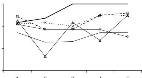
In selectingr LP was …rst or equal …rst in 20 of the 30 experiments. For the other
techniques the same result was: AIC 5; BIC 6; HQ 6; m5%r;n 9; and m1%r;n 7. Ranking the techniques on frequencies of correct selection of rfrom 1 (best) to 6 (worst), the average ranks were LP 1:97; AIC 4:9, BIC 2:77, HQ 2:8, m5%
r;n 2:93; and m1%r;n 3:33: The results were fairly consistent across the range of models although there were some patterns evident. Figure 1 shows a sample result for correct selection frequencies of
r in this case for n = 3; r = 2 and over the …ve models of i: LP tended to perform
better for the models with fewer deterministic processes (i = 3;4;5), the AIC was most frequently the worst, while m5%
r;n performed markedly better andm1%r;nperformed slightly better when i= 1;3 or5:
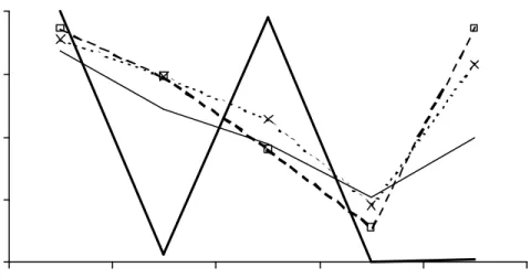
In selectingiLP was …rst or equal …rst in 13 of the 30 experiments. For the other
LP2:67;AIC3:03, BIC 1:9, and HQ2:17:The performance of LP was not consistent
over i; as LP came equal last 16 times (AIC 11 times, BIC 1 and HQ 0). Figure 2
shows the sample results for selection ofi:In this case the information criteria tended
to perform better when i= 1 or5; but poorly otherwise (particularly ati= 4). BIC
and HQ tend to over-select i = 5 when in fact i = 4: LP performs very well when
i = 1 or 3 (with relative frequencies near 1), but only occassionally selects correct i when i = 2;4; or 5: The better performance of the information criteria is due to
the treatment in the penalty function of the change in the number of parameters. The information criteria treat changes in the dimensions of ¯ and B symmetrically,
however the Laplace method distributes the changes among gamma functions and exponents. An alternative speci…cation of the prior for i could remove this problem, however the e¤ect diminishes with increased sample size.
The Monte Carlo results suggest that LP is useful for selectingr from the joint
distribution of (r; i); however when selecting iit performs well in only some cases.
7 An illustrative example: Interest rates.
In this section we demonstrate testing for the (r; i) for four U.S. treasury bill rates. The four interest rates are the 5 year (i5) and 1 year (i1) Treasury Bond rates (Capital
Market) and the 1 and 3 month and 1 and 5 year Treasury constant maturity rates (i30; i180; i1Y Rand i5Y R respectively). The data are annualised monthly rates for the
period January 1982 to January 1999 (T = 214).
These variables are useful for the study of the various theories for the term struc-ture of interest rates. Common implications of many of these theories is that, while the rates themselves may be integrated of order one, we would expect to …nd in this case, three cointegrating relations. It is unlikely that interest rates would contain lin-ear drifts suggesting i= 4 or5;however over the period in this sample rates showed
a clear downwards movement suggesting we may …nd i= 3. It is commonly assumed,
and there is strong empirical evidence in support of this assumption, that the rates enter the cointegrating relations through the spreads. With this assumption, choosing betweeni = 4and5depends upon our beliefs about the long run or equilibrium term
structure of the interest rates. If we believe the term structure to be ‡at, this would support i= 5;if we believe it is sloping (up or down) this would suggesti= 4:
Classical pretesting suggests each series is integrated of order one and we …nd an ECM with two lags of di¤erences is su¢cient to model the process. The residu-als in the ECM, particularly for the short rates, do not appear normal and this is largely due to excess kurtosis, however, following earlier studies using interest rates to demonstrate an application, such as Luukkonen, Ripatti and Saikkonen (1999), we ignore this feature as modelling this behaviour is outside the scope of this paper.
The information criteria select combinations of (r; i) of AIC (4;5), BIC (1;5)
5 and using m5%
r;n and m1%r;n; r = 2 is accepted. Posterior probabilities using LP suggest (r= 2; i= 3) to be the most likely combination with posterior probability of Pr (r = 2; i= 3jy) = 0:63. The conditional probabilities for ralso supportr = 2with Pr (r = 2ji = 3; y) = 0:68 and Pr (r= 2ji= 5; y) = 0:50. Conditioning on i= 3; m1% r;n supports r = 2whereas m5%
r;n supportsr = 4. The acceptance by the classical test of
r = 4when i= 3 at the 5% level of signi…cance is re‡ected in a Bayesian conditional
posterior probability ofPr (r= 4ji= 3; y) = 0:25:
8 Conclusion.
In this paper a method of …nding approximations to Bayes factors has been demon-strated for models of stochastic and deterministic processes of a cointegrating er-ror correction model. These approximations use both analytical integration and the Laplace method of approximating integrals. Although the Laplace method has been employed in many Bayesian studies, the approach in this article owes more to the classical literature on obtaining distributions of latent roots of covariance matrices. The Monte Carlo results suggest the Laplace approach performs well at selecting the number of stochastic trends when compared with the equivalent classical test statis-tics and information criteria. However, the approach does not perform consistently well when used to determine the deterministic processes in the data.
cointegrating vectors. As the object of interest is the cointegrating space, a prior is placed upon this parameter and this de…nes the implied prior for the elements in the cointegrating vectors.
9 Appendix.
The Laplace approximation.
Before applying the Laplace approximation to the integral in (8), de…ne by U = [U1U2] 2 O(n) the eigenvectors of A = D1¡1=2D2D¡11=2 such that A = U¤U0 and
¤ = diag(¸1(A); : : : ; ¸p(A)): Next let Dul = U0DlU for l = 0;1;2; H1 = U0¯ and since U 2O(n) then(¯0d¯) = (H10dH1)by invariance of (¯0d¯): Therefore
Z Vr;n f(¯)g(¯) (¯0d¯) = Z Vr;n f(UH1)g(UH1) (H10dH1)
where f(U H1) = jH10Du0H1j¡1=2jH10Du1H1j1=2: The Laplace approximation is then applied to this integral with respect to H1: This application requires the mode of f;
H1; and an expression for the Hessian of¡lnf atH1; ªr:
Maximising f > 0 is equivalent to minimising f¡2 = ¯¯H10D0uH1(H10Du1H1)¡1
¯ ¯. Note for am£m matrix E, jEj= ¦m
j=1¸i(E) = ¦mj=1¸i(U0EU): From an extension of the Poincaré separation theorem (see Schott 1997, p. 116)
minf¡2 = ¦rj=1¸n¡r+j¡D0uDu1¡1¢
Since D1¡1=2D0D1¡1=2 = In ¡ A; and ¸n¡r+j ¡ D0D¡11 ¢ = ¸n¡r+j ³ D¡11=2D0D¡11=2 ´ , then this equals 1¡¸j(A) = 1¡¸j(¤). Therefore, minf¡2 = ¦rj=1(1¡¸j(¤)) =
minjIr¡H1¤H1jwhich occurs atH1= [§Ir0]0where§Irmeans one of the2r matri-ces with zero o¤-diagonal elements and diagonal elements either +1 or -1. Therefore if H1= [Ir 0]0 for large T;
ct2r
Z
N(H1)
k(UH1) (H10dH1)
where N¡H1¢ denotes a neighbourhood of the matrixH1 (see Muirehead 1982, Ch. 9 p. 394 for a more detailed explanation of this point). This result will allow a simple form for the Hessian of ¡lnf(UH1) atH1:
First note that the Hessian of ¡lnf = 1
2lnjH10Du0H1j ¡ 21lnjH10D1uH1j has the form ªr= JH;hªHJH;h where ªH = ¡ @ 2lnf (@ vecH1)0(@ vecH1) = ª0¡ª1:
Using standard results for obtaining matrix di¤erentials (see Magnus and Neudecker, 1988), for l= 0;1 and using ¯=UH1;
ªl = h (¯0Dl¯)¡ 1 -³Dl¡Dl¯(¯0Dl¯)¡ 1 ¯0Dl ´i ¡h(¯0Dl¯)¡1¯0Dl-Dl¯(¯0Dl¯)¡1 i Kn;r
The nr£ r
2(2n¡r¡1)matrix JH;h contains the partial di¤erentials of H1 with respect to the free elements of H1 denoted by hij; dvec(hij)dvec(H). From Muirehead (1982), since H1 2Vr;n there exists a n£n orthogonal matrix H= [H1 :¡] given by
[H1:¡] = exp (X) = In+X + 1 2X 2+ 1 3!X 3+: : : ; (10) X = 2 6 6 4 X11 X12 ¡X120 0 3 7 7 5
where X and X11 are skew symmetric. IfH hasijth element hij andX has xij;then
hii = 1¡
1 2§
n
j=1x2ij+higher order terms, i·rand
hij = xij+higher order terms (i6=j); xij =¡xji (see James 1969 for details). In the neighbourhood N¡H1
¢
; X11 = 0 and X12 = 0: Di¤erentiate (10) once and set all remaining xij = 0 to obtain dvec(hdvec(H)ij) and thus the Jacobian from H1 to hij at H1 =H1.
10 Acknowledgements.
The authors would like to thank Herman van Dijk, Charles Bos, Frank Kleibergen, Brendan McCabe and participants of the workshop ‘Recent Advances in Bayesian Econometrics’ in Marseilles, June 2001 and two anonymous referees for useful discus-sion that has improved this paper.
11 References.
Akaike, H., 1974, A new look at the statistical model identi…cation, I.E.E.E. Trans-actions on Automatic Control, AC-19 (6): 716-723.
Anderson, G.A., 1965, An asymptotic expansion for the distribution of the latent roots of the estimated covariance matrix, Annals of Mathematical Statistics, 36, 1153-1173. Anderson, T.W., 1951, Estimating linear restrictions on regression coe¢cients for multivariate normal distributions, Annals of Mathematical Statistics, 22, 327-351. Bauwens, L. and M. Lubrano, 1996, Identi…cation restrictions and posterior densities in cointegrated Gaussian VAR systems, in Advances in Econometrics, Vol. 11B, Bayesian Methods Applied to Time Series Data, T.B. Fomby, ed., (JAI Press) 3-28. Boswijk, H. P., 1996, Testing identi…ability of cointegrating vectors, Journal of Busi-ness and Economic Statistics, 14, 153-160.
Billingsley, P. 1979, Probability and Measure (John Wiley and Sons, Inc., New York). Engle, R.F. and C.W.J. Granger, 1987, Co-integration and error correction: Repre-sentation, estimation and testing, Econometrica, 55, 251-276.
Geweke, J., 1996, Bayesian reduced rank regression in econometrics, Journal of Econo-metrics, 75, 121-146.
Granger, C.W.J., 1983, Cointegrated variables and error correction models, Discus-sion paper, University of California, San Diego.
Hannan, EJ and B.G. Quinn, 1979, The determination of the order of an autoregres-sion, Journal of the Royal Statistical Society:B, 41:2, 190–195.
James, A. T., 1954, Normal multivariate analysis and the orthogonal group, Annals of Mathematical Statistics, 25, 40-75.
James, A. T., 1969, Test of equality of the latent roots of the covariance matrix, in: P.R. Krishnaiah, ed., Multivariate Analysis, Vol. II (Academic Press, New York) 205–218.
Johansen, S., 1988, Statistical analysis of cointegration vectors, Journal of Economic Dynamics and Control, 12, 231-254.
Johansen, S., 1991, Estimation and hypothesis testing of cointegration vectors in Gaussian vector autoregressive models, Econometrica, 69, 111-132.
Johansen, S., 1995, Likelihood-based Inference in Cointegrated Vector Autoregressive Models (Oxford University Press, New York).
Kass, R.E. and A.E. Raftery, 1995, Bayes Factors, Journal of the American Statistical Association, 90, 773-795.
Kass, R.E. and S.K. Vaidyanathan, 1992, Approximate Bayes factors and orthogonal parameters, with application to testing equality of two binomial proportions, Journal of the Royal Statistical Society B, 54, 129–144.
Bayesian analysis of cointegration, Journal of Econometrics.
Kleibergen, F. and H.K. van Dijk, 1994, On the shape of the likelihood/posterior in cointegration models, Econometric Theory, 10, 514-551.
Larsson, R. and Villani, M. 2001, A distance measure between cointeration spaces, Economics Letters, 70, 21-27.
Lewis, S.M. and A.E. Raftery, 1997, Estimating Bayes factors via posterior simu-lation with the Laplace-Metropolis estimator, Journal of the American Statistical Association, 92, 648-655.
Lindley, D.V., 1980, Approximate Bayesian Methods, in: J.M. Bernardo, M.H. De-groot, D.V. Lindley, and A.M.F. Smith, eds., Bayesian Statistics, (Valencia, Spain: University Press).
Luukkonen, R, A. Ripatti and P. Saikkonen, 1999, Testing for a valid normalisation of cointegrating vectors in vector autoregressive processes, Journal of Business and Economic Statistics, 17, 195-204.
Magnus, J. R. and H. Neudecker, 1988, Matrix Di¤erential Calculus with Applications in Statistics and Econometrics (John Wiley and Sons, New York).
Muirhead, R. J., 1982, Aspects of Multivariate Statistical Theory (John Wiley and Sons, New York).
Royal Statistical Society, Series B, 57, 1, 99-138.
Raftery, A.E., 1994, Approximate Bayes factors and accounting for model uncertainty in generalized linear models, Technical report no. 255, Department of Statistics, University of Washington.
Schwarz, G., 1978, Estimating the dimension of a model, Annals of Statistics, 6:2, 461-464.
Strachan, R.W., 2003, Valid Bayesian estimation of the cointegrating error correction model, Journal of Business and Economic Statistics, 21:1, 185-195.
Strachan, R.W., and van Dijk, H. K. 2002, The value of structural information in the VAR, Discussion paper, University of Liverpool.
Tierney, L., R.E. Kass, and J.B. Kadane, 1989, Approximate marginal densities of nonlinear functions, Biometrika, 76, 425-433.
Tierney, L. and J.B. Kadane, 1986, Accurate approximations for posterior moments and marginal densities, Journal of the American Statistical Association, 81, 82-86. Villani, M., 2000, Aspects of Bayesian Cointegration. PhD. Thesis, University of Stockholm, Sweden.
Zellner, A., 1971, An Introduction to Bayesian Inference in Econometrics (John Wiley and Sons Inc., New York).
12 Figures. 0.25 0.50 0.75 1.00 1 2 3 4 5
Figure 1: The above …gures show the relative selection frequencies forr when n= 3; r = 2:The labels are given in the …gure and the x-axis shows the value of i.
0.00 0.25 0.50 0.75 1.00 1 2 3 4 5
Figure 2: The above …gures show the relative selection frequencies fori when n= 3; r = 2: The legend is given in Figure 1 and thex-axis shows the value of i.
0 . 0 0 0 . 2 5 0 . 5 0 0 . 7 5 1.00 1 2 3 4 5
LP
AIC
BIC
HQ
5%
1%
Figure 3: Legend for Figures 1 and 2. LP - Laplace approximation method; AIC, BIC and HQ are the information criteria and 5% and 1% are the classical trace tests.