Scalable data analytics techniques for summarizing spatial network-based observations

(1)

Scalable Data Analytics Techniques for Summarizing

Spatial Network-based Observations

A DISSERTATION

SUBMITTED TO THE FACULTY OF THE GRADUATE SCHOOL OF THE UNIVERSITY OF MINNESOTA

BY

Dev Oliver

IN PARTIAL FULFILLMENT OF THE REQUIREMENTS FOR THE DEGREE OF

Doctor of Philosophy

Advisor: Professor Shashi Shekhar

(2)

c

Dev Oliver 2014

(3)

Acknowledgements

I thank my advisor, Professor Shashi Shekhar, for his mentorship, support, and guid-ance throughout my Ph.D. I am truly grateful for the opportunities he has given me and the lessons he has imparted on me. I also thank all the professors who helped me over the years in classes including those who served on my committee: Professor Jaideep Sri-vastava, Professor Mohamed Mokbel, Professor Sudipto Banerjee, and Professor Vipin Kumar. Thank you for guiding my thesis and helping to shape my overall research.

I thank my collaborators from the National Geospatial-Intelligence Agency for giving me valuable insights into the societal applications of this research and for taking the time to provide feedback on many parts of this thesis. I will miss our regular meetings where we attempted to understand the world a little better through research.

I extend special thanks to Professor Shekhar’s Spatial Computing research group. Their beneficial comments have helped me with different aspects of my research and I really apreciate it. I thank Kim Koffolt for taking the time to provide feedback on my papers. I also thank Georganne Tolaas for her help during different milestones of this graduate program.

Lastly, I express my deepest appreciation to my wife Datra and our parents for their unwavering support during this journey.

(4)

Abstract

Summarizing spatial network-based observations (SSNO) entails finding a compact description or representation of large spatial or spatio-temporal datasets. For example, transportation planners and engineers may need to identify road segments that pose risks for pedestrians and require redesign. However, SSNO is computationally challenging for the following reasons: (1) There may be a large number of k-subsets of connected components in the network, (2) Patterns may not obey the monotonicity property, and (3) There may be a large number of candidates.

To address the challenge of the large number of k-subsets of connected components in the network, we explored the problem of spatial network activity summarization. In spatial network activity summarization (SNAS), we are given a spatial network and a collection of activities (e.g., pedestrian fatality reports, crime reports) and the goal is to find kshortest paths that summarize the activities. SNAS is important for applications where observations occur along linear paths such as roadways, train tracks, etc. Previous work has focused on either geometry or subgraph-based approaches (e.g., only one path), and cannot summarize activities using multiple paths. This work proposes a K-Main Routes (KMR) approach that discovers k shortest paths to summarize activities. To improve performance, KMR uses network Voronoi, divide and conquer, and pruning strategies. Experimental results on synthetic and real data show that KMR with our performance-tuning decisions yields substantial computational savings without reducing summary path coverage. We also present a case study comparing KMR with K-Means on real data.

To address the challenge ofpatterns not obeying the monotonicity property, we stud-ied the problem of geo-referenced time-series summarization. Given a set of regions with activity counts at each time instant (e.g., a listing of countries with number of mass protests or disease cases over time) and a spatial neighbor relation, geo-referenced time-series summarization (GTS) findsk-full trees that maximize activity coverage. GTS has important potential societal applications such as understanding the spread of political unrest, disease, crimes, etc. Previous approaches for spatio-temporal data mining detect anomalous or unusual areas and do not summarize activities. We propose a k-full tree

(5)

tion assignment) that leads to computational savings without affecting result quality. Analytical and experimental results show that the algorithmic refinement substantially reduces computational cost. We also present a case study that shows the output of our approach on Arab Spring data.

To address the challenge of a large number of candidates, we tackled the problem of significant linear hotspot discovery (SLHD). Given a spatial network and a collec-tion of activities (e.g., pedestrian fatality reports, crime reports), SLHD finds shortest paths in the spatial network where the concentration of activities is unusually high (i.e., statistically significant). SLHD is important for societal applications in transportation safety, public safety, or public health such as finding paths with significant concentra-tions of accidents, crimes, or diseases. SaTScan may miss many significant paths since a large fraction of the area bounded by circles for activities on a path will be empty. Previous network-based approaches only consider a small fraction of the network and only one significant network component (e.g., path). We propose novel algorithms for discovering statistically significant linear hotspots using the ideas of likelihood pruning, Monte Carlo speedup, and dynamic segmentation. We present a case study compar-ing the proposed approach with existcompar-ing techniques on real data. Experimental results show that the proposed algorithm, with our algorithmic refinements, yields substantial computational savings without reducing result quality.

The work in this thesis is the first step towards understanding the immense chal-lenges and novel applications of summarizing spatial network-based observations for transportation safety, public safety, disaster response, etc. In this thesis, we have for-mally modeled spatial and spatio-temporal network datasets and have begun to explore new data analytics techniques (e.g., K-Main Routes) that may have many uses in real-world applications. We conclude this thesis by exploring additional data summarization techniques for spatial networks, their computational challenges, and possible directions for future work.

(6)

List of Tables

1.1 Summarization framework for various data genres (Best in Color) . . . . 2

1.2 Sample crime report data in formats advocated by the US Department of Justice . . . 5

2.1 Examples of linear generators where observations occur along paths in the spatial network . . . 11

2.2 Shortest paths from Figure 2.1 (Activity Coverage refers to the number of activities on a path) . . . 12

2.3 Summarization framework for various data genres . . . 13

2.4 Initial seeds and final solutions of KMR . . . 38

3.1 Summarization framework for various data genres . . . 43

4.1 Number of paths explored by SRM with and without dynamic segmentation 82 5.1 Summarization framework with future work (Best in Color) . . . 96

(11)

List of Figures

1.1 Pedestrian fatalities occurring on arterials in Orange County, FL [1]. Activities such as pedestrian fatalities may be constrained by network connectivity and network distances (Best in color) . . . 1 1.2 An example of (a) spatial summarization (ellipses) and (b) spatial

net-work summarization (paths). . . 3 1.3 (a) Pedestrian at risk on a road without proper sidewalks [2] (b)

Pedes-trian fatalities occurring on arterials in Orlando, FL [1]. . . 4 1.4 (a) Types of crime hot spots (b) An example of a street-based (linear)

hotspot of crime in a major US city . . . 6 2.1 Example (a) Input and (b) Output of Spatial Network Activity

Summa-rization (Best in color). . . 12 2.2 (a) Pedestrian at risk on a road without proper sidewalks [2] (b)

Pedes-trian fatalities occurring on arterials in Orlando, FL [1]. . . 14 2.3 Two Methods of Summarizing Activities on a Network. . . 16 2.4 Execution trace of K-Main Routes (KMR). Circles represent nodes, lines

represent edges, and squares represent activities (Best in color). . . 23 2.5 An example of NOVA TKDE. Activity 10 gets assigned to summary path

hD, Ei because the shortest path hV, E, Fi from V to activity 10 goes through nodeE of summary path hD, Ei (Best in color). . . 25

(12)

the group are considered when choosing the new summary path which maximizes activity coverage. In this case, summary pathshA, B, Ci and

hC, B, Ai both maximize activity coverage based on activities 1,2,3,4,

and 5 so D-SPARE TKDE will choose one of these summary paths as the new representative for this group (Best in color). . . 26 2.7 SNAS instance resulting from Maximum Coverage instance for (a)

arbi-trary paths and (b) shortest paths. . . 29 2.8 Comparing KMR and Crimestat K-means output fork= 4 on pedestrian

fatality data from Orlando, FL [1] (Best in color). . . 32 2.9 Scalability of KMR with increasing number of nodes . . . 34 2.10 Scalability of KMR with increasing number of routes k . . . 35 2.11 Scalability of KMR with increasing (a) number of activities and (b) active

node ratio on synthetic data . . . 36 2.12 Example (a) Input and Output of (b) Top-k queries and (c) SNAS (Best

in color). . . 37 3.1 An example of (a) spatial summarization (ellipses) and (b) spatial graph

summarization (paths). . . 44 3.2 A geo-referenced time-series. . . 47 3.3 Spatio-temporal directed neighbor relationships. . . 48 3.4 Examples of spatio-temporal (ST) full trees from Figure 3.3 rooted atA1. 48 3.5 Example (a) input and (b) output of GTS (Best in color). . . 50 3.6 kFT Execution Trace (Best in color). . . 53 3.7 Voronoi Partition Assignment Example. A2 is assigned tohA1isinceA1

is a node on the shortest path fromV toA1, i.e.,V, A1, A2 (Best in color). 55 3.8 Effect of number of nodes on (a) synthetic and (b) real data . . . 56 3.9 Effect of number of time instants on (a) synthetic and (b) real data . . 57 3.10 Effect of number of trees on (a) synthetic and (b) real data . . . 57 3.11 kFT output on Arab Spring data from December 2010 to February 2011 [3]

(Best viewed in color). . . 59 4.1 Simplified example of Significant Linear Hotspot Discovery where activity

information is aggregated by edge (Best in color). . . 62

(13)

trian fatalities occurring on arterials in Orlando, FL [1]. A large fraction of the bounding circles (e.g., C1, C2) of significant routes are empty (Best in color). . . 62 4.3 Simplified example (a) Input, where activities are summarized by total

count per edge (b) Output of Linear Intersecting Paths (LIP) [4], and (c) Output of Constrained Minimum Spanning Trees (CMST) [5] (Best in color). . . 65 4.4 Example of dynamic segmentation where paths between activities at the

sub-edge level are considered. . . 66 4.5 Execution trace of Na¨ıve Significant Route Miner (Na¨ıveSRM). Circles

represent nodes and lines represent edges (Best in color). . . 72 4.6 (a) Example of Likelihood Pruning. Since we know the upper-bound

likelihood for hN1, N2, N5i is 4, we can avoid calculating the shortest paths hN1, N2, N5, N6i and hN1, N2, N5, N7i for θ = 5. (b) Example of Monte Carlo Speedup. (Best in color). . . 75 4.7 Example of Dynamic Segmentation where the network structure is altered

such that new nodes are formed at the locations of activities and new edges are added to connect these nodes. Paths such ashA1,A2,A3,A4,

A5,A6,A7imay be evaluated directly for statistical significance. In this example, the number of nodes exceeds the number of activities. . . 79 4.8 Example of (a) the hierarchical filter and (b) the active node filter for

dynamic segmentation. Shortest paths between activities are determined by stitching together (1) shortest paths between nodes in the statically segmented network with (2) paths between activities and the start and end of their original edges. Shortest path hA1, A10i is calculated by stitching togetherhA1, N2i,hN2, N5i, and hN5, A10i. The active node filter refines (1) by only considering shortest paths between active nodes. (Best in color). . . 90

(14)

dynamic segmentation), and SaTScan’s output for a p-value threshold of 0.15 andθ= 1.75 on pedestrian fatality data from Orlando, FL [1] (Best in color). . . 91 4.10 Scalability with increasing (a) number of nodes, (b) likelihood ratio

thresh-oldθ, (c) p-value threshold, and (d) activities . . . 92 4.11 Colored dots are part of chance clusters identified by DBScan [6] on a

complete spatial randomness dataset (Best in color). . . 92 5.1 Ring-Shaped Summary based on domain concepts and theories in

En-vironmental Criminology. There exists a constant tension between the offenders desire to divert attention from his or her home base and the desire to travel no further than necessary to commit crimes [7] (Best in Color) . . . 99 5.2 Classification of Summarization featuring Natural Geographic Concepts 99

(15)

Chapter 1

Introduction

Many human activities are centered around spatial infrastructure networks, such as transportation, oil/gas-pipelines, and utilities (e.g., water, electricity, telephone). Thus, activity reports such as pedestrian fatalities or crime reports may often use network based location references, e.g., street addresses such as 200 Blizzard Street, Happyville, DQ 94401. The spatial interaction among activities at nearby locations may also be constrained by network connectivity and network distances (e.g., shortest paths along roads or train networks) rather than geometric distances (e.g. Euclidean or Manhattan distances) used in traditional spatial analysis.

Figure 1.1: Pedestrian fatalities occurring on arterials in Orange County, FL [1]. Ac-tivities such as pedestrian fatalities may be constrained by network connectivity and network distances (Best in color)

(16)

Figure 1.1 shows an example of 487 pedestrian fatalities occurring on a road network in Orange County, FL from 2001 - 2011 (Orlando is located in Orange County) [1]. As can be seen, the observations are constrained by network connectivity and network distances and are not occurring arbitrarily in space.

1.1 Summarization Framework

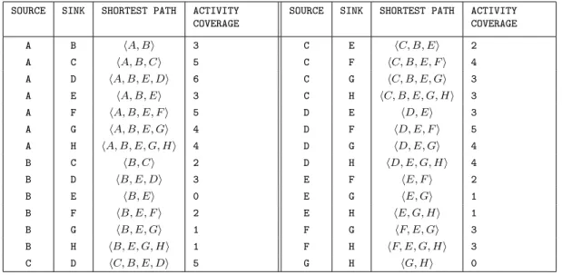
Summarizing spatial network-based observations entails finding a compact description or representation of large spatial or spatio-temporal network datasets where the observa-tions (e.g., pedestrian fatality reports, crime reports), are centered around the network. The process typically involves defining a set of groups, finding a representative for each group, and reporting a statistic for each group (e.g., sum, mean, likelihood ratio). These notions differ depending on the genre of the data being summarized.

Table 1.1: Summarization framework for various data genres (Best in Color)

Table 1.1 presents a summarization framework for different genres of data such as relational tables, spatial datasets, spatial networks, and geo-referenced time-series. An example of relational table summarization, is the GROUP BY clause in SQL that is used to group rows having common values to report SQL aggregation functions such as mean and standard deviation [8]. The group definition in this case is a partition of rows and the group representation is distinct values of attributes such as age-groups, citizenship, income-group, etc. Vector space is an alternate view of summarization where the groups may be a partition of vectors or significant groups of vectors, the

(17)

group representative may be a vector or a basis function, and the statistic may be an aggregate property (e.g., count, sum, mean) or a significance metric (e.g., p-value, likelihood ratio, confidence interval).

Spatial Euclidean summarization includes heat maps and hotspot analysis. Heat maps provide a graphical representation of data in which individual values contained in a matrix are represented as colors. The group definition for heat maps might include a set of pixels and the group representation may be a subset of these pixels. Hotspots are a special kind of partitioned pattern where objects in hotspot regions have high similarity in comparison to one another and are dissimilar to all the objects outside the hotspot [9]. These spatial summarizations are based on spatial point locations where the group definition is a partition of space and the groups could be represented by points, polygons, ellipses, or line-strings. An example of a spatial summarization is given in Figure 3.1(a) where incidents of crime in a major US city are shown as dots and the spatial (Euclidean) summarization is represented using ten ellipses. The spatial summarization technique used in this case was K-Means [10].

(a) (b)

Figure 1.2: An example of (a) spatial summarization (ellipses) and (b) spatial network summarization (paths).

Spatial network summarization defines groups based on a partition of a graph and represents groups using nodes, paths, trees, etc. For example, the thicker lines in Figure 3.1(b) illustrate a summarization technique that uses linear representatives or paths to represent each partition [11]. Here four paths are used to summarize the incidents of crime (dots) that are on the spatial network (i.e., the road network).

Summarization of the last data genre listed in the table, geo-referenced time-series summarization, defines groups based on a partition of a geo-referenced time series and may represent groups using spatio-temporal (ST)-nodes, ST-paths, or ST-heaviest full

(18)

trees.

1.2 Illustrative Application Domains

Two representative application domains are transportation safety and environmental criminology, notably, the areas of preventing pedestrian fatalities and crime analysis.

Preventing Pedestrian Fatalities: According to a recent policy report, more than 47,700 pedestrians were killed in the United States from 2000 and 2009 [2]. More than 688,000 pedestrians were injured over the same time period, which is equivalent to a pedestrian being struck by a vehicle every 7 minutes. Pedestrian fatalities have increased in many places, including 15 of the country’s largest metro areas, even as overall traffic deaths have fallen [2].

(a) (b)

Figure 1.3: (a) Pedestrian at risk on a road without proper sidewalks [2] (b) Pedestrian fatalities occurring on arterials in Orlando, FL [1].

Domain experts attribute pedestrian fatalities largely to the design of streets, which have been engineered for speeding traffic with little or no provision for people on foot, in wheelchairs or on bicycles [2]. Daily activities have shifted away from main streets towards higher speed arterials based on the emphasis on traffic movement. This has resulted in more than half of fatal pedestrian crashes occurring on these wide, high capacity and high-speed thoroughfares. Typically designed with four or more lanes and high travel speeds, arterials are not built with pedestrians in mind (Figure 4.2(a)). They lack sidewalks, crosswalks (or have crosswalks spaced too far apart), pedestrian refuges, street lighting, and school and public bus shelters [2].

The consequences of this lack of basic infrastructure are fatal. For example, forty percent of fatalities occurred where no crosswalk was available [2]. Figure 4.2(b) shows

(19)

a map of pedestrian fatalities that occurred on Orlando roads from 2000 - 2009. Trans-portation planners and engineers need tools to assist them in identifying which fre-quently used road segments/stretches pose risks for pedestrians and consefre-quently should be redesigned. Road segments/stretches that pose risks to pedestrians may be concep-tualized as linear concentrations because the generation model of pedestrian fatalities is inherently linear, i.e., they occur on roads.

Crime Analysis: Environmental criminology is the study of crime, criminality, and victimization as they relate to particular places and to the way that individuals and organizations shape their activities spatially [12]. Environmental criminology is used by law enforcement to develop an understanding of the spatial distributions (e.g., high activity places or hot-spots) of crime activities as well as location-based factors af-fecting activities using analytical techniques, e.g., crime mapping, and analytical tools such as CrimeStat [13]. Environmental criminology is also used to assist police depart-ments by enabling the design of patrol routes and providing street-based descriptions of crime attractors and generators (e.g., a bar after closing time) [14]. Table 1.2 illus-trates real crime report datasets collected by police departments in formats advocated by the US Department of Justice. Crime reports provide locations using symbolic sys-tems (e.g., street addresses, highway-mile markers) as well as numerical syssys-tems (e.g., latitude/longitude), which refer to a point.

Table 1.2: Sample crime report data in formats advocated by the US Department of Justice

ID OFFENCE TYPE DATE TIME ADDRESS

96 Burglary 1/14/2006 1530 16950 GRAND AVE

477 Auto Theft 8/2/2006 2042 7950 W FAIRVIEW 1960 633 Narcotic Drug Laws 11/2/2006 1200 12950 CLEVELAND DR

Environmental criminology has several spatial theories such as Routine Activity Theory (RAT) [15] and Crime Pattern Theory (CPT) [16]. RAT suggests that the location of a crime is related to the criminal’s frequently visited areas and CPT extends this theory on a spatial model. Crime is not spread evenly across maps but instead is concentrated in some areas and absent in others [17]. This knowledge is used everyday by people and is seen in the way they avoid some places and seek out others. Police also use this understanding to make decisions about how to allocate scarce resources based

(20)

in part on where police demand is highest. Officers are told to be attentive in certain areas but are not given guidance in other areas where crime is scarce [17].

The various areas of concentrated crime (i.e., hotspots) are typically studied in terms of places, neighborhoods, and streets [17]. For places, an explanation as to why crime events occur at specific locations is sought. For neighborhoods, analysts look at large areas and ask questions such as “Which areas are claimed by gangs and which areas are not?”. Street-based analysis deals with crimes that occur over small stretched areas such as streets or blocks and examples include street drug dealing, prostitution, and robberies of pedestrians [17]. Figure 1.4 illustrates these various types of hotspots.

(a) (b)

Figure 1.4: (a) Types of crime hot spots (b) An example of a street-based (linear) hotspot of crime in a major US city

The National Institute of Justice, which is the research, development and evaluation agency of the U.S. Department of Justice, has pointed out that “commonly available mapping programs make it easy to identify hot spot places or hot spot areas, but do not make linear hotspots easy to identify. Most clustering algorithms, unfortunately, will show areas of concentration even when a line is the most appropriate dimension” [17].

1.3 Computational Challenges

Summarizing spatial network-based observations is computationally challenging for the following reasons: (1) There may be a large number of k-subsets of connected compo-nents in the network, (2) Patterns may not obey the monotonicity property, and (3) There may be a large number of candidates.

(21)

a set ofk connected components such as shortest paths is computationally challenging. This is due to the fact that if k connected components are selected from all connected components in a spatial network, there are a large number of possibilities for large k, i.e., n_k

, where n is the number of connected components. This is because different subsets of k connected components could be overlapping or have the same connected components. For disjoint components, the problem would be relatively less computa-tionally challenging. However, due to overlapping connected components, the general problem remains extremely challenging.

Patterns may not obey the monotonicity property: Given an interest measure to model domain semantics, patterns in the spatial network may not obey the monotonicity property. For example, if the interest measure is to maximize activity coverage, a connected component such as a path or tree with no activity may belong to a larger region with many activities. This makes it more challenging to prune subsets as all connected components may have to be considered. Determining appropriate interest measures for various domains is important in capturing domain semantics. Examples of possible interest measures include maximum activity coverage, minimum average distance, likelihood ratio, etc. Summarization based on maximizing activity coverage works well in domains such as transportation safey because it captures areas with the most activity (e.g., pedestrian fatalities) whereas summarization based on likelihood ratio works well in domains such as epidemiology because it captures regions where the concentration of activities is unusually high (i.e., statistically significant).

Large number of candidates: The search space itself may have potentially large number of candidates. For example, in a transportation planning scenario, there may be as many as 1016_{shortest paths in a given dataset with hundreds of millions of activities} or road network nodes. For large roadmaps such as the 100 million road-segments in the US, this results in prohibitive shortest path computation times.

1.4 Thesis Contributions

The main contributions of this thesis address the three challenges of summarizing spatial network-based observations outlined in the previous section.

(22)

First, the challenge of there being alarge number of k-subsets of connected compo-nents in the network was addressed by studying the problem of spatial network activity summarization [18, 11]. We proposed a K-Main Routes (KMR) approach that discovers

k shortest paths to summarize activities. KMR generalizes K-means for network space but uses shortest paths instead of ellipses to summarize activities. To improve perfor-mance, KMR used network Voronoi, divide and conquer, and pruning strategies. We presented a case study comparing KMR’s network-based output (i.e., shortest paths) to geometry-based outputs (e.g., ellipses) on pedestrian fatality data. Experimental results on synthetic and real data showed that KMR with our performance-tuning decisions yielded substantial computational savings without reducing summary path coverage.

Second, we examined the problem of geo-referenced time-series summarization (GTS) to address the challenge where patterns may not obey the monotonicity property [19]. We proposed a k-full tree (kFT) approach for GTS which featured an algorithmic re-finement that led to computational savings without affecting result quality. The algo-rithmic refinement is Voronoi partition assignment for partitioning regions. Analytical and experimental results showed that the algorithmic refinement substantially reduced computational cost. We also presented a case study that showed the output of our approach on Arab Spring data.

Finally, addressing thelarge number of candidates challenge was done by exploring the problem of significant linear hotspot discovery [20]. We proposed novel algorithms for discovering statistically significant linear hotspots using the ideas of likelihood prun-ing, Monte Carlo speedup, and dynamic segmentation. We presented a case study comparing the proposed approach with existing techniques on real data. Experimental results showed that the proposed algorithm, with our algorithmic refinements, yielded substantial computational savings without reducing result quality.

1.5 Thesis Organization

This thesis is organized as follows: In Chapter 2, we tackle the challenge of there be-ing a large number of k-subsets of connected components in the network through the problem of spatial network activity summarization and our proposed K-Main Routes (KMR) algorithm. We examine the challenge where subsets of patterns may not obey

(23)

the monotonicity property by studying the problem of geo-referenced time-series sum-marization and our proposed K-Full Tree (KFT) approach in Chapter 3. Chapter 4 discusses the challenge of a large search space due to the large number of candidates by exploring the significant linear hotspot discovery problem and our proposed approaches. Finally, in Chapter 5, we summarize our findings and identify related areas that remain open for future research.

(24)

Chapter 2

A K-Main Routes Approach to

Spatial Network Activity

Summarization

2.1 Introduction

Spatial network activity summarization (SNAS) has important applications in domains where observations occur along linear paths in the network. Table 2.1 provides ex-amples of such applications where the generative model of observations is inherently linear. For example, transportation planners and engineers may need to identify road segments/stretches that pose risks for pedestrians and require redesign [2]; crime an-alysts may look for concentrations of crimes along certain streets to guide law en-forcement [17]; and hydrologists may try to summarize environmental change on water resources to understand the behavior of river networks and lakes [21].

Informally, the SNAS problem can be defined as follows: Given a spatial network, a collection of activities and their locations (e.g., placed on a node or an edge), and a desired number of paths k, find a set of k shortest paths that maximizes the sum of activities on the paths (counting activities that are on overlapping paths only once) and a partitioning of activities across the paths. Depending on the domain, an activity may be the location of a pedestrian fatality, a carjacking, a train accident, etc. SNAS

(25)

Table 2.1: Examples of linear generators where observations occur along paths in the spatial network

Linear Generator Example

Arterial roads Pedestrian fatalities have largely "occurred along arterial roadways (i.e., wide, high capacity and high-speed roads) that were dangerous by design, streets engineered for speeding traffic with little or no provision for people on foot, in wheelchairs, or on bicycles" [2]. Transportation planners and engineers may need to identify frequently used road segments/stretches that pose risks for pedestrians and require redesign.

Crime-prone streets Crime analysts look for linear concentrations of crime (linear generators and attractors) such as speeding, street drug dealing, drunk driving, etc. to guide law enforcement [17].

Water resource changes in rivers

Environmental engineers may try to summarize environmental change on water resources to understand the behavior of river networks and lakes [21]

Transportation route disaster

"A snowstorm in Hungary brought drifts 10 feet (3 meters) high and violent gusts of wind, forcing thousands of people to spend the night in their cars or in emergency shelters after being stranded on a major highway" [22]. Emergency managers may find it useful to summarize the locations of stranded cars on highways (e.g., the M1 highway in Hungary) to better understand how to allocate resources.

Railroads Transportation officials are interested in understanding

railroad accidents (e.g., derailing) to improve safety and reduce cost [23].

assumes that every path is a shortest path because in applications such as transportation planning, the aim is usually to help people to arrive at their destination as fast as possible. Figures 4.1(a) and 4.1(b) illustrate an input and output example of SNAS, respectively. The input consists of eight nodes, seven edges (with edge weights of 1 for simplicity), eleven activities, and k= 2, indicating that two routes and groups are desired. Table 2.2 shows the shortest paths for the spatial network in Figure 2.1 and their respective activity coverages (i.e., the sum of activities on each shortest path). The output contains two shortest paths and two groups of activities. The shortest paths are representatives for each group and each shortest path maximizes the activity coverage for the group it represents. For example, route hA, B, Ci is the representative for the group comprised of activities 1,2,3,4, and 5, and route hD, E, Fi is the representative for the group comprised of activities 6,7,8,9,10,and 11.

Finding a set ofkshortest paths that maximizes the number of activities on selected paths is computationally challenging. This is due to the fact that if k shortest paths are selected from all shortest paths in a spatial network, there are a large number of possibilities for large k, i.e., n_k

(26)

(a) (b)

Figure 2.1: Example (a) Input and (b) Output of Spatial Network Activity Summariza-tion (Best in color).

because different subsets of k shortest paths could be overlapping or have the same shortest paths. For disjoint paths, the problem would be relatively less computationally challenging. However, due to overlapping paths, the general problem of SNAS is NP-complete and its proof is provided in this chapter (Section 2.4).

Table 2.2: Shortest paths from Figure 2.1 (Activity Coverage refers to the number of activities on a path)

SOURCE SINK SHORTEST PATH ACTIVITY COVERAGE

SOURCE SINK SHORTEST PATH ACTIVITY COVERAGE A B hA, Bi 3 C E hC, B, Ei 2 A C hA, B, Ci 5 C F hC, B, E, Fi 4 A D hA, B, E, Di 6 C G hC, B, E, Gi 3 A E hA, B, Ei 3 C H hC, B, E, G, Hi 3 A F hA, B, E, Fi 5 D E hD, Ei 3 A G hA, B, E, Gi 4 D F hD, E, Fi 5 A H hA, B, E, G, Hi 4 D G hD, E, Gi 4 B C hB, Ci 2 D H hD, E, G, Hi 4 B D hB, E, Di 3 E F hE, Fi 2 B E hB, Ei 0 E G hE, Gi 1 B F hB, E, Fi 2 E H hE, G, Hi 1 B G hB, E, Gi 1 F G hF, E, Gi 3 B H hB, E, G, Hi 1 F H hF, E, G, Hi 3 C D hC, B, E, Di 5 G H hG, Hi 0

2.1.1 A Framework for Data Summarization

Data summarization is an important concept in data mining that entails techniques for finding a compact description or representation of a dataset. The process typically involves defining a set of groups, finding a representative for each group, and reporting a statistic for each group (e.g., sum, mean, standard deviation). These notions differ

(27)

depending on the genre of the data being summarized. Table 3.1 presents a summa-rization framework for three genres of data. An example of the first, relational table summarization, is the GROUP BY clause in SQL that is used to group rows having com-mon values to report SQL aggregation functions such as mean and standard deviation. The group definition in this case is a partition of rows and the group representation is distinct values of attributes such as age-group, income-group, etc.

Table 2.3: Summarization framework for various data genres

Data Genre Group Definition

(Partitioning Criteria)

Group Representation Choices

Statistic Relational Table (a set

of rows)

a partition of rows Distinct values of attributes (e.g., age-group) sum, count, mean, etc. Spatial (Euclidean Space)

a partition of space points, polygons, ellipses, line-strings

sum, count, mean, etc. Spatial Network

(Neighbor Relationship)

a partition of a graph node, path, tree, subgraph

sum, count, mean, etc.

The second genre is spatial Euclidean summarization, which includes heat maps and hotspot analysis. Heat maps provide a graphical representation of data in which individual values contained in a matrix are represented as colors. The group definition for heat maps might include a set of pixels, and the group representation may be a subset of these pixels. Hotspots are a special kind of partitioned pattern where objects in hotspot regions have high similarity in comparison to one another and are dissimilar to all the objects outside the hotspot [9]. These spatial summaries are based on spatial point locations where the group definition is a partition of space and the groups could be represented by points, polygons, ellipses, or line-strings.

In this work we explore the third genre, spatial network summarization, which defines groups based on partitioning a network and may represent groups using nodes, paths, trees, etc.

2.1.2 An Illustrative Application Domain: Preventing Pedestrian Fa-talities

To illustrate the applicability of SNAS, we focus on the problem of pedestrian fatalities. According to a recent policy report, more than 47,700 pedestrians were killed in the United States from 2000 and 2009 [2]. More than 688,000 pedestrians were injured over

(28)

the same time period, which is equivalent to a pedestrian being struck by a vehicle every 7 minutes. Pedestrian fatalities have increased in many places, including 15 of the country’s largest metro areas, even as overall traffic deaths have fallen [2].

(a) (b)

Figure 2.2: (a) Pedestrian at risk on a road without proper sidewalks [2] (b) Pedestrian fatalities occurring on arterials in Orlando, FL [1].

Domain experts attribute pedestrian fatalities largely to the design of streets, which have been engineered for speeding traffic with little or no provision for people on foot, in wheelchairs or on bicycles [2]. Daily activities have shifted away from main streets towards higher speed arterials based on the emphasis on traffic movement. This has resulted in more than half of fatal pedestrian crashes occurring on these wide, high capacity and high-speed thoroughfares. Typically designed with four or more lanes and high travel speeds, arterials are not built with pedestrians in mind (Figure 4.2(a)). They lack sidewalks, crosswalks (or have crosswalks spaced too far apart), pedestrian refuges, street lighting, and school and public bus shelters [2].

The consequences of this lack of basic infrastructure are fatal. For example, forty percent of fatalities occurred where no crosswalk was available [2]. Figure 4.2(b) shows a map of pedestrian fatalities that occurred on Orlando roads from 2000 - 2009. Trans-portation planners and engineers need tools to assist them in identifying which fre-quently used road segments/stretches pose risks for pedestrians and consefre-quently should be redesigned. Road segments/stretches that pose risks to pedestrians may be concep-tualized as linear concentrations because the generation model of pedestrian fatalities is inherently linear, i.e., they occur on roads. This chapter presents an approach for identifying linear concentrations of activities such as pedestrian fatalities in a spatial network.

(29)

2.1.3 Related Work

Summarizing activities by grouping is a significant research area in data mining. Pre-vious techniques have generally been geometry-based [10, 24, 25, 26, 27] or network-based [28, 29, 30, 31, 32, 33, 34, 35, 36, 37].

In geometry-based summarization, partitioning of spatial data is based on grouping similar points distributed in planar space where distance is calculated using Euclidean distance, not network distance. Such techniques focus on the discovery of the geometry (e.g., circle, ellipse) of high density regions [17] and include K-Means [10], K-medoid [24, 25], P-median [26] and Nearest Neighbor Hierarchical Clustering [27]. These methods do not consider the underlying spatial network; they group spatial objects that are close in terms of Euclidean distance but not close in terms of network distance. Thus, they may fail to group activities that occur on the same street.

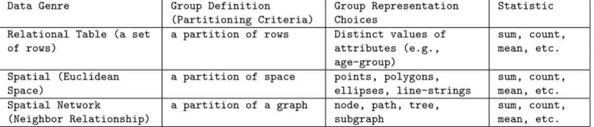
In network-based summarization, spatial objects are grouped using network (e.g., road) distance. Existing methods of network-based summarization such as Mean Streets [28], Maximal Subgraph Finding (MSGF) [29], and Clumping [30, 31, 32, 33, 34, 35, 36, 37] group activities over multiple paths, a single path/subgraph, or no paths at all. Mean Streets [28] finds anomalous streets or routes with unusually high activity levels. It is not designed to summarize activities over k paths because the number of high crime streets returned is always relatively small. MSGF [29] identifies the maximal subgraph (e.g., a single path, k = 1) under the constraint of a user specified length and cannot summarize activities when k > 1. The Network-Based Variable-Distance Clumping Method (NT-VCM) [37] is an example of the clumping technique [30, 31, 32, 33, 34, 35, 36, 37]. NT-VCM groups activities that are within a certain shortest path distance of each other on the network; in order to run NT-VCM, a distance threshold is needed.

An example output of NT-VCM is shown in Figure 2.3(b). The threshold distance for NT-VCM is the unit distance between activities 8 and 11. However, NT-VCM is not designed to summarize activities usingk paths because the grouping of activities is based on the given distance threshold. As such, activities 1, 2, 3, 4, and 5, which occur on the same street would not belong to the same group, given this threshold distance.

Network distance may also be applied to certain geometry-based techniques such as K-Means [10]. Figure 2.3(c) shows an example of the ellipses output by K-Means

(30)

(a) Input (b) NT-VCM Output [37]

(c) K-Means Output (network dis-tance)

Figure 2.3: Two Methods of Summarizing Activities on a Network.

using network distance. The left ellipse groups activities 1, 2, 3, 6, 7, 8, and 11 whereas the right ellipse groups activities 4, 5, 9, and 10. Even when generalized with network distances, these methods output point-based or ellipsoid-based groups, not paths. The objective of network-based K-Means (e.g., minimize the within-cluster sum of squares) is different from that of SNAS (e.g., maximize activity coverage), which explains their difference in output.

Previously, we proposed K-Main Routes (KMR) using inactive node pruning as a heuristic for summarizing activities in a spatial network [11]. We demonstrated the correctness of inactive node pruning, experimentally evaluated KMR, and presented a case study comparing the output of network based with geometry based summariza-tion. However, our previous approach was limited in terms of performance and use of heuristics without proof of NP-completeness.

2.1.4 Contributions

In this chapter, we show that SNAS is NP-complete and propose two additional tech-niques for improving the performance of KMR: 1) Network Voronoi activity Assignment, which allocates activities to the nearest summary path, and 2) Divide and conquer Summary PAth REcomputation, which calculates the new summary path of each group using only group nodes. Applying these two performance-tuning techniques results in significant computational savings. Specifically, our research contributions are as follows:

(31)

• We introduce a summarization framework demonstrating how different genres of data may be summarized.

• We show that SNAS is NP-complete.

• We propose two new techniques for improving the performance of K-Main Routes (KMR): Network Voronoi activity Assignment (NOVA TKDE) and Divide and conquer Summary PAth REcomputation (D-SPARE TKDE).

• We analytically demonstrate the correctness of NOVA TKDE and D-SPARE TKDE.

• We analyze the computation costs of KMR.

• We present a case study comparing KMR with geometry-based summarization techniques on pedestrian fatality data.

• We test the performance and scalability of KMR using both synthetic and real-world data sets and demonstrate the computational efficiency of our performance-tuning strategies.

2.1.5 Scope and Outline of the chapter

This work focuses on summarizing discrete activity events (e.g., pedestrian fatalities, crime reports) associated with a point on a network. This does not imply that all activities must necessarily be associated with a point in a street. Furthermore, other network properties such as GPS trajectories and traffic densities of road networks [38] are not considered. The objective function used in SNAS is based on maximizing the activity coverage of summary paths, not on minimizing the distance of activities to summary paths. The summary paths are shortest paths but other spatial constraints are not considered (e.g., nearest neighbors) [39]. Additionally, it is assumed that the number of activities on the road network is fixed and does not change over time. A dynamically changing number of activities is presently beyond the scope of this research. The chapter is organized as follows: Section 4.2 presents the basic concepts and problem statement of SNAS. Section 2.3 explains KMR, NOVA TKDE, and

(32)

case study comparing KMR with other summarization techniques. The experimental evaluation is covered in Section 4.6. Section 4.7 presents a discussion and Section 4.8 concludes the chapter and previews future work.

2.2 Basic Concepts and Problem Statement

This section introduces several key concepts in SNAS and presents a formal problem statement.

2.2.1 Basic Concepts

We define our basic concepts as follows:

Definition 1. A spatial network G = (N, E) consists of a node set N and an edge set E, where each element u in N is associated with a pair of real numbers (x, y)

representing the spatial location of the node in a Euclidean plane [40]. Edge set E is a subset of the cross product N ×N. Each element e= (u, v) in E is an edge that joins node u to node v.

An example of a spatial network is shown in Figure 2.1(a). In the figure, circles represent nodes and lines represent edges. A road network is an example of a spatial network where nodes represent street intersections and edges represent streets.

Definition 2. An activity set A is a collection of activities. An activity a∈ A is an object of interest associated with only one edge e∈E or one node n∈N.

In Figure 2.1(a), activities are represented as squares. In transportation planning, an activity may be the location of a pedestrian fatality; in crime analysis, an activity may be the location of a theft; and in disaster response an activity may be the location of a request for relief supplies.

Definition 3. A summary path set Pˆ is a collection of summary paths where each pathpi∈Pˆ is a shortest path. Asummary pathimposes a partitioning on an activity

set A such that network distance(a, pi)≤network distance(a, pj) ∀pj ∈P ,ˆ ∀a∈A.

Figure 2.1(b) shows two summary pathshA, B, CiandhD, E, Fi. Activities 1,2,3,4,

(33)

activities 6,7,8,9,10 and 11 form a partition around hD, E, Fibecause they are closer tohD, E, Fi. Here the network distance between an activity and a path,

i.e., network distance(a, pi), is the network distance between aand the closest node in pi.

Definition 4. The activity coverage AC(p) of a path p is the sum of activities having network distance = 0 from an edge e ∈p. The activity coverage AC(P) of a set of paths P is the sum of activities across individual paths pi in set P, having

network distance = 0 from each edge e∈P, counting activities that are covered several times only once. If two paths share an edge, the activities on that edge are only counted once.

For example, in Figure 2.1(a) the activity coverage of the shortest path from node

A to node B is 3 because there are 3 activities occurring on that path. Likewise, the activity coverage of the shortest path from node Dto node F is 5 because there are 5 activities occurring on hD, E, Fi. If the set of paths are hA, B, Ci and hD, E, Fi, then the activity coverage is 10 because there are 10 activities on all the edges of the paths inP. If the set of paths arehA, B, Ci and hA, Bi, then the activity coverage is 5. Note that the activities on edge AB are only counted once even though AB is an edge in both paths.

2.2.2 Problem Statement

The problem of spatial network activity summarization (SNAS) can be expressed as follows:

Given:

1. A spatial network G = (N, E) with weight function w(u, v) ≥ 0 for each edge

e= (u, v)∈E (e.g., network distance),

2. A set of activities A and their locations (e.g., a node or an edge),

3. A desired number of summary paths, k, wherek≥ 1.

(34)

1. A summary path set of size k,

2. A partitioning of activities across these summary paths.

Objective: Maximize the activity coverage of each summary path for the group it represents.

Constraints:

1. Each summary path is a shortest path between its end-nodes,

2. Each activity a∈A is associated with only one edge e∈E.

The spatial network input for SNAS is defined in Definition 8. The activities input are objects of interest in the spatial network such as the locations of pedestrian fatalities. The k input represents the desired number of summary paths. The output for SNAS is a summary path set of size k and a partitioning of activities across the paths. The summary paths are representatives for each group and each summary path maximizes the activity coverage for the group it represents. The optimal solution for SNAS may not be unique and this is shown in lemma 1.

Example. The network in Figure 4.1(a) can be viewed as a road network, com-posed of streets (edges) and intersections (nodes) with eleven activities (squares). The aim is to find two routes and two groups of activities; the routes are representatives for each of the groups. In a transportation planning scenario, identifying such routes would guide street redesign efforts to reduce the risk of pedestrian fatalities (e.g., adding sidewalks, crosswalks, pedestrian refuges, street lighting, etc.). In Figure 4.1(b), route

hA, B, Ciis the representative for the group comprised of activities 1,2,3,4, and 5; and route hD, E, Fi is the representative for the group comprised of activities 6,7,8,9,10 and 11.

2.3 Spatial Network Activity Summarization

This section describes the computational structure of SNAS. It also describes the K-Main Routes (KMR) algorithm and its performance-tuning decisions Network Voronoi activity Assignment, Divide and conquer Summary PAth REcomputation, and Inactive Node Pruning.

(35)

2.3.1 Computational Structure of SNAS

In SNAS, the optimal solution may not be unique. Additionally, among the optimal solutions there are some where every path starts and ends at active nodes. These properties are formally shown via Lemmas 1 and 2.

Definition 5. An active edge is an edge e ∈ E that has 1 or more activities. An

active node is a node u joined by an active edge or a node that has one or more activities, or both. An inactive node is a node that is not joined by any active edges.

EdgesABand BC in Figure 2.1(a) are active edges because they each have at least one activity and nodes A,B,C,D,E, F, and Gare all active nodes because they are all joined by active edges. By contrast, Node H is an inactive node because it is not joined by any active edges.

Lemma 1. The optimal solution for SNAS may not be unique.

Proof. There may be multiple solutions for different values of k. For example, given

k = 1 in Figure 2.1(a) where all eleven activities are members of the same group, the summary path could be hA, B, E, Di or hD, E, B, Ai, since both these paths have a maximum activity coverage of 6 based on the one group. Given k = 2 and the groups shown in Figure 4.1(b), the summary paths could behA, B, CiandhD, E, FiorhC, B, Ai

and hF, E, Di as both sets of paths have a maximum activity coverage of 11 based on their respective groups.

Lemma 2. Among the optimal solutions for SNAS, there exist optimal solutions where every path starts and ends at active nodes.

Proof. Let’s begin with an arbitrary optimal solution. Let p be a shortest path that starts or ends with inactive nodes. If inactive nodes that start or end p are removed such that p starts and ends with active nodes, the resulting subpathp′ is still optimal in terms of activity coverage, because no active edges were removed. p′ is also still a shortest path due to the optimal substructure of shortest paths wherein subpaths of shortest paths are shortest paths [41]. In other words, eliminating inactive nodes from the beginning and end of a shortest path does not reduce coverage and does not split the path. KMR takes advantage of this property to achieve computational savings.

(36)

2.3.2 K-Main Routes Algorithm

Algorithm 1 presents the pseudocode for the proposed K-Main Routes (KMR) approach. The basic structure of KMR resembles that of K-Means [10] in terms of selecting initial seeds, formingkgroups, and updating the representative of each group until the assign-ments no longer change. Line 1 of Algorithm 1 selects all shortest paths P that start and end with active nodes (inactive node pruning). Next, k paths from P are selected as initial summary paths, which are the “seeds” for KMR (line 2). The algorithm then proceeds in two main phases. First, it forms k groups by assigning each activity to its closest summary path (line 4). Then, it updates the summary path of each group by calculating the shortest path that maximizes activity coverage (line 5). Assigning and updating repeat until the summary paths no longer change and the final summary paths and groups are returned (line 8).

Algorithm 1 K-Main Routes (KMR) Algorithm Input:

1) a spatial network G= (N, E), 2) a set of activities A,

3) a number of routesk,

4) mode1∈ {naive, N OV A T KDE}, 5) mode2∈ {naive, D-SP ARE T KDE}

Output:

A summary path set of sizekand a partitioning of activities across these summary paths, where the objective is to maximize the activity coverage of each summary path for the group it represents.

Algorithm:

1: P ←shortest paths between active nodes of G

2: Pˆ ←k summary paths∈P;stableGroups←f alse; 3: while notstableGroupsdo

4: Phase 1: currentGroups←AssignActivities

-T oSummaryP aths(G,A,k, ˆP,mode1) 5: Phase 2: ˆP′←RecomputeSummaryP aths

(G,A,k,currentGroups,mode2) 6: if Pˆ= ˆP′ thenstableGroups←true

7: Pˆ ←Pˆ′

8: return currentGroups

(37)

network shown has eight nodes, seven edges, and eleven activities. For illustration purposes, we choosehA, BiandhD, Eias initial summary paths,k= 2, and set all edge weights to 1.

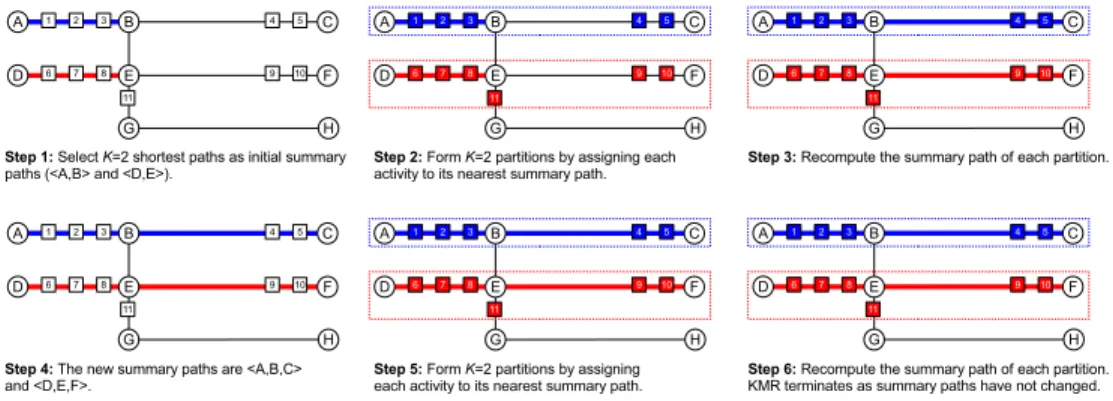
Figure 2.4: Execution trace of K-Main Routes (KMR). Circles represent nodes, lines represent edges, and squares represent activities (Best in color).

In step 2 of Figure 4.5, two groups are formed by assigning each activity to its closest summary path. In this example, activities 1, 2, 3, 4, and 5 are assigned to the summary path hA, Bi, and activities 6, 7, 8, 9, 10 and 11 are assigned to the summary pathhD, Ei. The groups are highlighted with dashed lines. In cases where the distance between an activity and several summary paths is equal, the activity is assigned to one of those summary paths at random.

Once groups are formed, the summary paths of each group have to be recalculated, as shown in step 3. In this case, the new summary paths (shown in step 4) arehA, B, Ci

and hD, E, Fi. These summary paths are chosen because they further maximize the activity coverage. In other words, based on the activities of each group, summary paths

hA, B, Ci andhD, E, Fi have maximum activity coverage.

Step 5 repeats step 2 using the new summary paths hA, B, Ci and hD, E, Fi. The groups formed in this case are indicated by the dashed lines. Step 6 involves another recalculation of the summary paths to further maximize the activity coverage. The summary paths that are recalculated do not change and as a result, the algorithm terminates. We now discuss each phase of KMR in detail.

(38)

Phase 1: Assign activities to nearest summary paths

In this phase, k groups are formed by assigning each activity to its closest summary path. Algorithm 2 presents the pseudocode for the activity assignment algorithm which has two modes: naive and NOVA TKDE. The naive mode enumerates all the distances between every activity and summary path, and then assigns each activity to its closest summary path. NOVA TKDE, by contrast, avoids the enumeration that is done in the naive mode while still providing correct results.

Performance-Tuning for Phase 1: The Network Voronoi activity Assignment (NOVA TKDE) technique is a faster way of assigning activities to the closest summary path. Consider a virtual node, V, that is connected to every node of all summary paths by edges of weight zero. The basic idea is to calculate the distance from V to all active nodes and discover the closest summary path to each activity. The shortest path from

V to each activitya will go through a node in the summary path that is closest toa. NOVA TKDE starts by initializing all the relevant data structures. Line 5 of Algo-rithm 2 initializes the virtual node V connected to each node of all summary paths by edges of weight 0. Line 6 initializes the Openlist and Tnodes toV and the Closedand Tactivities to the empty set. NOVA TKDE then expands every node in the Open list

based on how close it is to the summary paths; closer nodes get expanded first. Once a node nis expanded, it is moved to the Closedlist (line 8). Next, each ofn′sneighbors

xi ∈/ Closedis examined, and Tnodes is updated withxi’s distanceand sp information,

where xi.distance is the network distance of xi from the nearest summary path, and xi.sp isxi’s assigned summary path. xi.distance is calculated by adding n.distance to

the distance of edge (n, xi) (line 9). Ifxi is not inOpen, it is then added to theOpen

list (line 10).

Once NOVA TKDE finds activities on an edge connecting node n to a summary path, it records the activity distance to that summary path. Every activityai that is on

edge (n, xi) is examined, andTactivitiesis updated withai’sdistanceandspinformation,

where ai.distance is the network distance ofai from the nearest summary path (based

on n), and ai.sp is the assigned summary path of ai. Next, an activity is assigned to

a summary path (line 12). If the activity was previously assigned to another summary path, it is removed from that path before being assigned to the new summary path. Once all active nodes have been added to the Closed list, or the Open list is empty,

(39)

NOVA TKDE’s main loop is stopped (line 13). If unassigned activities remain due to no connectivity to summary paths, these activities are randomly assigned to any summary path ∈ Pˆ (line 14). NOVA TKDE then returns the current groups and terminates (line 15).

Figure 2.5: An example of NOVA TKDE. Activity 10 gets assigned to summary path

hD, Ei because the shortest pathhV, E, Fifrom V to activity 10 goes through nodeE

of summary path hD, Ei (Best in color).

An example of NOVA TKDE activity assignment is shown in Figure 2.5. Virtual node V is connected by zero weight edges to nodes A and B of summary path hA, Bi

and nodes D and E of summary path hD, Ei (Algorithm 2, line 5). Activity 10 gets assigned to summary pathhD, Eibecause the shortest pathhV, E, FifromV to activity 10 goes through node E of summary path hD, Ei. Similarly, activity 5 gets assigned to summary path hA, Bi because the shortest path hV, B, Ci from V to activity 5 goes through node B of summary path hA, Bi.

Phase 2: Recompute summary paths

In phase 2, the summary path of each group is recomputed so as to further maximize activity coverage (i.e., the number of activities covered by the set of paths). Algorithm 3 presents the pseudocode, which has two modes: naive and D-SPARE TKDE. The naive mode enumerates the shortest paths between all active nodes in the spatial network while D-SPARE TKDE considers only the set of shortest paths between the active nodes of a group, which gives the correct results.

Performance-Tuning for Phase 2: The Divide and Conquer Summary PAth REcomputation (D-SPARE TKDE) technique chooses the summary path of each group with maximum activity coverage but only considers the set of shortest paths between the nodes of a given group (Algorithm 3, lines 8-9). D-SPARE TKDE assumes rich

(40)

connectivity and otherwise may return a summary path going outside a given frag-ment. If maxP ath is null after looking at the shortest paths in a given group, ci ∈ currentGroups, the shortest path which has the maximum activity coverage based on the activities inci is selected asmaxP ath(lines 10-12). maxP athis then added to ˆP as

the new summary path for ci (line 13). Once all groups ci∈currentGroups have been

considered, ˆP, which contains the summary paths with maximum activity coverage for each group, is returned.

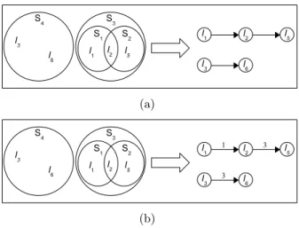
Figure 2.6: An example of D-SPARE TKDE. Only shortest paths between nodes in the group are considered when choosing the new summary path which maximizes activity coverage. In this case, summary paths hA, B, Ci and hC, B, Ai both maximize activity coverage based on activities 1,2,3,4,and 5 so D-SPARE TKDE will choose one of these summary paths as the new representative for this group (Best in color).

Figure 2.6 shows an example of D-SPARE TKDE where the given group consists of activities 1,2,3,4,and 5, and summary pathhA, Bi. The goal of D-SPARE TKDE is to choose a new summary path that maximizes activity coverage for every group based on the activities of each group. In this case, summary paths hA, B, Ci and hC, B, Ai both maximize activity coverage based on activities 1,2,3,4,and 5, so D-SPARE TKDE will choose one of these summary paths as the new representative for this group.

KMR with Inactive Node Pruning Performance-Tuning: We also applied a pruning strategy to K-Main Routes to improve its performance. Rather than checking all shortest paths, inactive node pruning considers only paths between active nodes, thereby reducing the total number of paths considered (Algorithm 1, line 1). For ex-ample, Figure 2.1(a) shows a spatial network with eight nodes, seven edges, and eleven activities. The active nodes in this network are A, B, C, D, E, F, and G. Without inactive node pruning, the number of shortest paths considered would be 56 because there are eight nodes, and the shortest path between each node and every other node is considered. With inactive node pruning, the number becomes 42, as only the shortest paths between the seven active nodes are considered.

(41)

2.4 Theoretical Analysis

In this section, we present a proof of NP-Completeness for spatial network activity summarization. We also present proofs of correctness for our proposed performance-tuning techniques.

2.4.1 Proof of NP-Completeness

For simplicity, we begin by defining a generalized, decision version of SNAS where the set of paths might be arbitrary and show this problem to be NP-complete. We then present a proof sketch showing that the decision version of SNAS with shortest paths is also NP-complete.

Definition 6. Decision version of SNAS:

INSTANCE: A spatial network G = (N, E) with weight function w(u, v) ≥ 0 for each edge e = (u, v) ∈ E, a set of activities A and their locations, a set of paths P, a desired number of routes k, and a bound B ∈Z+, where Z+ denotes the set of positive integers.

QUESTION: Does P contain a cardinality k subset P′ of P, i.e., a subset P′ ⊆

P with |P′_|₌ _k _and _AC₍_P′₎ _≥ _B_{, where} _AC₍_P′₎ _{denotes the activity coverage of} _P′_?

Theorem 1. SNAS is NP-complete.

Proof. The process of devising an NP-completeness proof for a decision problem Π consists of the following four steps [42]:

1. showing that Π is in NP,

2. selecting a known NP-complete problem Π′,

3. constructing a transformation f from Π to Π′, and

4. proving that f is a (polynomial) transformation

In step 1, to show that SNAS ∈NP, assume that a certificate and a number B are given. The certificate consists of a spatial network G = (N, E) with weight function

(42)

desired number of routes k, and a cardinality k subset P′ of P, i.e., a subset P′ ⊆ P

with |P′| = k. We can then verify in polynomial time whether AC(P′) ≥ B because

AC(P′) involves counting the number of activities inP′.

Step 2 selects the Maximum Coverage problem [43] as a known NP-complete problem Π′. Although the optimization version of Maximum Coverage [43] is known to be NP-Hard, its decision version is NP-Complete. The decision version is specified as follows:

INSTANCE: A number k and a collection of sets S = S1, S2, . . . , Sm , where Si ⊆ {l1, l2, . . . , ln}, and a bound B∈Z+, whereZ+ denotes the positive integers.

QUESTION: Does S contain a subset S′ ⊆S of sets such that |S′| ≤ k and the number of covered elements

S Si∈S′ Si ≥B?

Steps 3 and 4 construct a transformation f from Π to Π′ and prove that f is a (polynomial) transformation. The reduction entails a polynomial time transformation of the input of Maximum Coverage to the input of SNAS followed by a polynomial time transformation of the output of SNAS to the output of Maximum Coverage. The input of Maximum Coverage may be transformed to the input of SNAS using the following steps:

1. Impose a total order T O onn elements inL={l1, l2, ..., ln}.

2. Convert each element in L into a node with one activity.

3. Convert each set Si to a pathPi .

• Add edge (lj, lj+1) ∀ j∈1...|Si|.

The transformation computation time is dominated by the polynomial step of sorting the elements in Si using T O. Thus it is easy to see that the entire transformation

is indeed polynomial. Consider an instance of the Maximum Coverage problem as shown in Figure 2.7(a) where L = {l1, l2, l3, l5, l6}, k = 2, S1 = {l1, l2}, S2 = {l2, l3},

S3 ={l1, l2, l3}, and S4 ={l5, l6}. The resulting instance of SNAS would thus be P =

{(l1 → l2), (l2 → l3), (l1 → l2 → l3), (l5 → l6)},k= 2, A={a1, a2, a3, a5, a6}, and ActivityN ode={a1(l1), a2(l2), a3(l3), a5(l5), a6(l6)}.

Next, we convert the instance of SNAS output to an instance of Maximum Coverage output. The transformation, which is also polynomial, is as follows:

(43)

(a)

(b)

Figure 2.7: SNAS instance resulting from Maximum Coverage instance for (a) arbitrary paths and (b) shortest paths.

• For each k path Pi produced by SNAS, convert the activities on the path into

elements and form a set Si.

The candidate solutions for the instance of SNAS shown in Figure 2.7(a) are (l1 → l2 → l3) and (l5 → l6). The resulting instance of the Maximum Coverage output would be S1 ={l1, l2, l3}and S2 ={l5, l6}.

The reduction of Maximum Coverage to SNAS is a polynomial time reduction since the input of Maximum Coverage can be reduced to SNAS in polynomial time, and the output of SNAS can be reduced to Maximum Coverage in polynomial time.

Since SNAS belongs to the class of NP and a known NP-complete problem is reduced to it, the decision version of SNAS is NP-complete.

We now present a proof sketch that the decision version of SNAS where the set of paths are shortest paths is also NP-complete. We follow the same construction as before but assign a cost for the edge (li, lj) to be j−i(Figure 2.7(b)). This step ensures that

all paths generated by construction are shortest paths.

2.4.2 Correctness of Performance-Tuning Decisions

We prove the correctness of inactive node pruning, NOVA TKDE, and D-SPARE TKDE as follows:

(44)

Theorem 2. Inactive node pruning is a correct filtering method.

Proof. A filtering method is considered correct if it does not exclude all optimal solu-tions. By Lemma 2, among the optimal solutions for SNAS, there exist optimal solutions where every path starts and ends at active nodes. Since inactive node pruning does not prune out any path that starts and ends at active nodes, no such optimal solutions will be pruned. Thus, inactive node pruning is correct.

Theorem 3. Network Voronoi activity Assignment (NOVA TKDE) is a correct activity assignment method, i.e., it assigns every activity to the nearest summary path.

Proof. An activity assignment method is considered correct if it assigns every activity to its nearest summary path. Let each activity be located at a particular node n∈N

and let a virtual source node V be added to G= (N, E) such that V is connected by an edge of zero weight to each node in the set of summary paths, ˆP. The correctness of NOVA TKDE can be argued in a similar fashion to that of Dijkstra’s algorithm [41], where each active node containing activity a is connected to V via the nearest node

n∈Pˆ. Sinceais assigned to the summary pathp∈Pˆ containing noden, it is assigned to the nearest summary path. Thus, NOVA TKDE is correct.

Theorem 4. Divide and Conquer Summary Path Recomputation (D-SPARE TKDE) is a correct summary path recomputation method, i.e., it returns a shortest path with maximum activity coverage for a given group c∈C.

Proof. A summary path recomputation method is considered correct if it returns a shortest path with maximum activity coverage for a given groupc∈C. In recomputing a summary pathp∈c, all shortest paths between nodes in a given groupcare considered. Thus, the optimal solution, i.e., the shortest path with maximum activity coverage in

c, will not be filtered and will be returned. Thus, D-SPARE TKDE is correct.

Lemma 3. AssignActivitiesToSummaryPaths terminates on all inputs

Proof. AssignActivitiesToSummaryPaths has two modes: naive and NOVA TKDE. The naive mode terminates on all inputs because there are a finite number of distances considered in assigning activities to the nearest summary path since there are a finite number of activities and summary paths. If the distances between an activity a and