ANALYSIS OF PROCESS DATA
WITH SINGULAR SPECTRUM
METHODS
by
Marlize Barkhuizen
Thesis presented in partial fulfilment of the requirements for the Degree
of
Masters of Science in Engineering
(Chemical Engineering)
in the Department of Process Engineering
at the University of Stellenbosch
Supervised by:
Prof C Aldrich
STELLENBOSCH
SOUTH AFRICA
DECEMBER 2003
DECLARATION
I, the undersigned, hereby declare that the work contained in this thesis is my own original work and that I have not previously in its entirety or in part submitted it at any university for a degree.
SYNOPSIS
The analysis of process data obtained from chemical and metallurgical engineering systems is a crucial aspect of the operating of any process, as information extracted from the data is used for control purposes, decision making and forecasting. Singular spectrum analysis (SSA) is a relatively new technique that can be used to decompose time series into their constituent components, after which a variety of further analyses can be applied to the data. The objectives of this study were to investigate the abilities of SSA regarding the filtering of data and the subsequent modelling of the filtered data, to explore the methods available to perform nonlinear SSA and finally to explore the possibilities of Monte Carlo SSA to characterize and identify process systems from observed time series data.
Although the literature indicated the widespread application of SSA in other research fields, no previous application of singular spectrum analysis to time series obtained from chemical engineering processes could be found.
SSA appeared to have a multitude of applications that could be of great benefit in the analysis of data from process systems. The first indication of this was in the filtering or noise-removal abilities of SSA. A number of case studies were filtered by various techniques related to SSA, after which a number of neural network modelling strategies were applied to the data. It was consistently found that the models built on data that have been prefiltered with SSA
outperformed the other models.
The effectiveness of localized SSA and auto-associative neural networks in performing nonlinear SSA were compared. Both techniques succeeded in extracting a number of nonlinear components from the data that could not be identified from linear SSA. However, it was found that localized SSA was a more reliable approach, as the auto-associative neural networks would not train for some of the data or extracted nonsensical components for other series.
Lastly a number of time series were analysed using Monte Carlo SSA. It was found that, as is the case with all other characterization techniques, Monte Carlo SSA could not succeed in correctly classifying all the series investigated. For this reason several tests were used for the classification of the real process data.
In the light of these findings, it was concluded that singular spectrum analysis could be a valuable tool in the analysis of chemical and metallurgical process data.
OPSOMMING
Die analise van chemise en metallurgiese prosesdata wat verkry is vanaf chemiese of metallurgiese ingenieursstelsels is ‘n baie belangrike aspek in die bedryf van enige proses, aangesien die inligting wat van die data onttrek word vir prosesbeheer, besluitneming of die bou van prosesmodelle gebruik kan word. Singuliere spektrale analise is ‘n relatief nuwe tegniek wat gebruik kan word om tydreekse in hul onderliggende komponente te ontbind. Die doelwitte van hierdie studie was om ‘n omvattende literatuuroorsig oor die ontwikkeling van die tegniek en die toepassing daarvan te doen, beide in die ingenieursindustrie en in ander navorsingsvelde, die navors van die moontlikhede van SSA aangaande die verwydering van geraas uit die data en die gevolglike modellering van die skoon data te ondersoek, ‘n ondersoek te doen na sommige van die beskikbare tegnieke vir nie-lineêre SSA en laastens ‘n studie te maak van die potensiaal van Monte Carlo SSA vir die karakterisering en identifikasie van data verkry vanaf prosesstelsels.
Ten spyte van aanduidings in die literatuur dat SSA wydverspreid toegepas word in ander navorsingsvelde, kon geen vorige toepassings gevind word van SSA op chemiese prosesse nie.
Dit wil voorkom asof die chemiese nywerhede groot baat kan vind by SSA van prosesdata. Die eerste aanduiding van hierdie voordele was in die vermoë van SSA om geraas te verwyder uit tydreekse. ‘n Aantal tipiese gevalle is ondersoek deur van verskeie benaderings tot SSA gebruik te maak. Nadat die geraas uit die tydreekse van die toetsgevalle verwyder is, is neurale netwerke gebruik om die prosesse te modelleer. Daar is herhaaldelik gevind dat die modelle wat gebou is op data wat eers deur SSA skoongemaak is, beter presteer as die wat slegs op die onverwerkte data gepas is.
Die effektiwiteit van lokale SSA en auto-assosiatiewe neurale netwerke om nie- lineêre SSA toe te pas is ook vergelyk. Albei tegnieke het daarin geslaag om nie- lineêre hoofkomponente van die data te onttrek wat nie geïdentifiseer kon word deur die lineêre benadering nie. Daar is egter gevind dat lokale SSA ‘n meer betroubare tegniek is, aangesien die
auto-assosiatiewe neurale netwerke nie op sommige van die datastelle wou leer nie en vir ander tydreekse sinnelose hoofkomponente onttrek het.
Laastens is ‘n aantal tydreekse geanaliseer met behulp van Monte Carlo SSA. Soos met alle ander karakteriseringstegnieke, kon Monte Carlo SSA nie daarin slaag om al die tydreekse wat ondersoek is korrek te identifiseer nie. Om hierdie rede is ‘n kombinasie van toetse gebruik om die onbekende tydreekse te klassifiseer.
In die lig van al hierdie bevindinge, is die gevolgtrekking gemaak dat singuliere spektrale analise ‘n waardevolle hulpmiddel kan wees in die analise van chemiese en metallurgiese prosesdata.
This is not the end.
It is not even the beginning of the end.
But it is the end of the beginning.
ACKNOWLEDGEMENTS
My heavenly Father for giving me the abilities, strength and opportunities to come this far. My study leader, Prof Chris Aldrich, for his patient guidance, continued support and invaluable input in my work.
My parents for believing in me and always having a word of support, encouragement and praise, as the need arose.
My friends for showing interest, giving advice and ‘just being there’, even though my work was largely Greek to them.
Fred for promising everything would turn out all right (it did). Mintek for their continued financial support and interest in my work.
TABLE OF
CONTENTS
TABLE OF CONTENTS v
LIST OF FIGURES viii
LIST OF TABLES xv
1. INTRODUCTION 1
2. LITERATURE REVIEW 3
2.1ORIGINS OF SINGULAR SPECTRUM ANALYSIS... 3
2.2SSA COMPARED TO OTHER SPECTRAL TIME SERIES ANALYSIS TECHNIQUES... 4
2.2.1 Fourier analysis 4
2.2.2 Wavelet analysis 4
2.2.3 Maximum Entropy Method (MEM) 4
2.2.4 Multi-taper method (MTM) 5
2.3TRENDS ANALYSIS WITH SSA... 5
2.3.1 Climatology and paleoclimatology 5
2.3.2 Biosciences 8
2.3.3 Economics 10
2.3.4 Geophysics 11
2.3.5 Engineering applications 12
2.3.6 Solar physics 14
2.4OTHER APPLICATIONS OF SSA ... 15
2.4.1 Process modelling and forecasting 15
2.4.2 Change point detection 16
3. METHODOLOGY 18
3.1 BASIC SINGULAR SPECTRUM ANALYSIS... 18
3.1.1 Decomposition stage 19
3.1.2 Reconstruction stage 22
3.1.3 Literature review on embedding and window length 23
3.1.4 Noise reduction 24
3.1.5 Interpretation of eigenelements 25
3.1.6 Prediction 25
3.2 MULTICHANNEL SINGULAR SPECTRUM ANALYSIS... 25
3.3 MONTE CARLO SSA... 26
3.3.1 Monte Carlo in the literature 28
3.3.2 General approach to Monte Carlo SSA 30
3.3.3 Generation of surrogate data 31
3.3.4 Choosing a test statistic 32
3.4 NONLINEAR SINGULAR SPECTRUM ANALYSIS... 33
3.4.1 Nonlinear Principal Component Analysis 33
3.4.2 Localized Principal Component Analysis 36
3.5 OTHER APPROACHES TO SSA... 38
3.5.1 Multi-scale singular spectrum analysis 38
3.5.2 Random lag singular spectrum analysis 38
3.5.3 Approximate projectors 38
4. FILTERING OF DATA WITH SSA 39
4.1IDENTIFICATION OF PROCESS SYSTEM... 39
4.2FLOW BETWEEN TWO NONINTERACTING TANKS IN SERIES... 42
4.2.1 Generation of series and performing SSA 42
4.2.2 Modelling of data series 44
4.2.3 Influence of window length 45
4.2.4 Reconstructed attractor 47
4.3CARBON-IN-LEACH PROCESS... 48
4.3.1 Background 48
4.3.2 Grouping of eigenvalues 50
4.3.3 Filtering of data 52
4.4BASE METAL FLOTATION PLANT – ROUGHER, CLEANER AND SCAVENGER CIRCUITS... 54
4.4.1 Background 54
4.4.2 Embedding of plant data 55
4.4.3 Modelling of the cleaner, rougher and scavenger 58
4.5BASE METAL FLOTATION PLANT – RECOVERY IN SCAVENGER CIRCUIT... 61
4.5.1 Background and performance of SSA 61
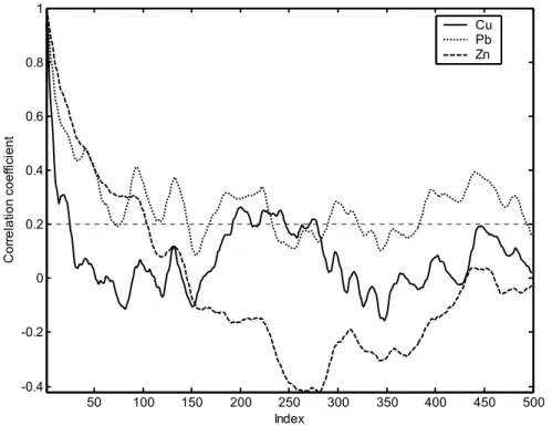
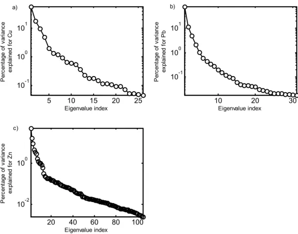
4.5.2 Modelling of the Cu, Pb and Zn in the scavenger 63
4.6LEAD FLOTATION PLANT... 66
4.6.1 Background and singular spectrum analysis 66
4.6.2 Modelling 68
4.7COMPARISON BETWEEN BEHAVIOUR OF SSA WHEN ANALYSING RED VS. WHITE NOISE... 70
4.7.1 Sine wave contaminated by various noise series 71
4.7.2 SSA of sine wave 73
4.7.3 Alternative techniques to deal with coloured noise 73
4.8SUMMARY... 74
5. NONLINEAR SSA 75
5.1FLOW IN A SERIES OF TANKS... 75
5.1.1 Background 75
5.1.2 Linear and localized SSA of four tanks in series process 76
5.1.3 Auto-associative neural network 82
5.2ELECTROCHEMICAL NOISE PROCESS... 83
5.2.1 Background 83
5.2.2 Linear and localized SSA of electrochemical noise process 87
5.2.3 Auto-associative neural network analysis 94
5.3SUMMARY... 96
6. MONTE CARLO SSA 97
6.1ARTIFICIAL DATA SETS WITH KNOWN PROPERTIES... 97
6.1.1 Properties of artificial time series 97
6.1.2 Characterization of time series 100
6.2.1 Background 115
6.2.2 Monte Carlo simulations 116
6.3AUTOCATALYSIS IN A CONTINUOUS STIRRED TANK REACTOR... 118
6.3.1 Simulation of time series 118
6.3.2 Characterization of time series by use of Monte Carlo SSA 120
6.4SUMMARY... 123
7. APPLICATIONS OF MONTE CARLO SSA 124
7.1COMPOSITION OF SCAVENGER CIRCUIT FROM BASE METAL FLOTATION PLANT... 124
7.1.1 Background and SSA 124
7.1.2 Characterization of time series based on Monte Carlo SSA 126
7.2AVALANCHING BEHAVIOUR OF PARTICLES... 131
7.2.1 Background 131
7.2.2 Experimental set-up and resulting time series 132
7.2.3 Singular spectrum analysis results 135
7.2.4 Classification of flow behaviour by means of Monte Carlo SSA 138
7.2.5 Investigation of correlation dimension 144
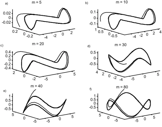
7.2.6 Reconstructed attractors 147
7.3SUMMARY... 150
8. CONCLUSIONS 152
REFERENCES 154
INDEX 165
APPENDIX A SOFTWARE DEVELOPED 166
A.1MATLAB SOFTWARE... 166
A.2PROGRAMMING CODE OF SSA_CALC TOOLBOX... 166
LIST OF
FIGURES
Figure 3.1 Four basic steps of SSA, namely embedding of time series, decomposition by use of PCA or SVD, grouping of components and reconstruction of additive components... 19 Figure 3.2 Autocorrelation function of artificial series, x, and three random, white noise
surrogates generated from this series. ... 28 Figure 3.3 Flow diagram illustrating the general approach to Monte Carlo SSA in that
surrogate data sets with similar parameters than that of the original time series are generated and by using a test statistic, both are tested against the postulated null hypothesis... 28 Figure 3.4 Illustration of the differences between (a) linear and (b) nonlinear time series where (a) can be fitted by a linear hyperplane, but (b) requires a curved approach. ... 34 Figure 3.5 Layout of neural network for nonlinear principal component analysis. ... 35 Figure 3.6 Flow diagram of algorithm of auto-associative neural network analysis... 36 Figure 3.7 Illustration of localized nonlinear approach to singular spectrum analysis compared to the linear approximation. ... 37 Figure 3.8 Diagrammatical presentation of steps involved in localized SSA approach to time series. ... 37
Figure 4.1 Modelling strategies (A) - (D), where the original time series is predicted in strategy A, the time series reconstructed by SSA predicted in strategy B, the individual components extracted by SSA predicted in strategy C and the reconstructions obtained from multichannel SSA predicted in strategy D. ... 41 Figure 4.2 Actual response (solid line) of a 2nd order system to a pulsed input (dashed line) and simulated observations (‘+’ markers)... 42 Figure 4.3 Autocorrelation function for two-tank series. ... 43 Figure 4.4 Eigenspectrum for the response (solid line) shown in Figure 4.2. ... 43 Figure 4.5 Reconstruction of the observed time series (dotted line), true process dynamics (solid line) and observations (‘+’ markers)... 44 Figure 4.6 Prediction of the output flow rate from the two-tank system in section 4.2. Values in parentheses in the legend are the r2-values associated with the models. ... 45 Figure 4.7 Eigenspectra obtained from singular spectrum analysis of two tanks in series time series by using different window lengths... 46 Figure 4.8 Enlargement of sections of eigenspectra obtained from singular spectrum analysis of two tanks in series time series by using different window lengths. ... 47 Figure 4.9 Reconstructed attractor of two tanks in series time series for different window lengths of the embedding window. ... 48 Figure 4.10 Simulated carbon-in-leach process with noisy observations (‘+’-markers) and true dynamics (broken line). ... 49 Figure 4.11 Autocorrelation function of carbon-in-leach simulated CSTR process. ... 50
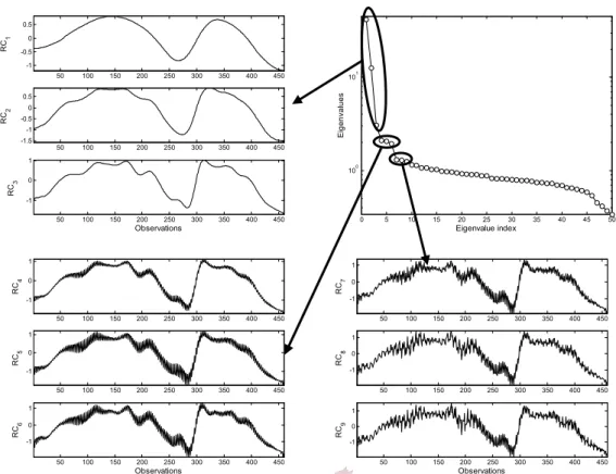
Figure 4.12 Eigenspectrum of the data in Figure 4.10 and the cumulative reconstructed time series (RC1–RC9) associated with the first 9 eigenvalues... 51
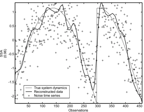
Figure 4.13 Individually reconstructed components for the first nine eigenvectors extracted from the carbon-in-leach cascaded CSTR process... 52 Figure 4.14 Moving average filters of filter window sizes of 5, 11 and 15 which were built on the noise-corrupted time series (solid lines) are compared with the original clean signal (dotted line). Correlation of the filtered series with the original time series is supplied in
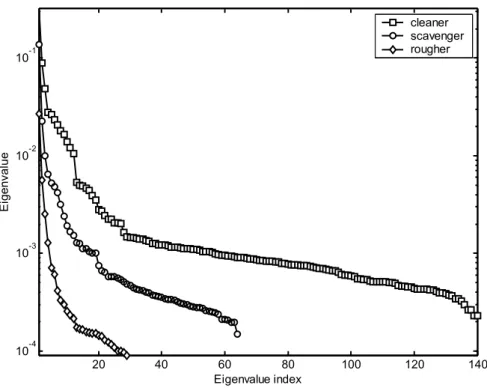
brackets. ... 53 Figure 4.15 Filtering of the carbon-in-leach cascaded CSTR process obtained by using SSA and a reconstruction with only three components (solid line), in comparison with the true process dynamics (dotted line) and the noisy time series on which the filtering was applied (‘+’-markers)... 54 Figure 4.16 Time series observations of the copper froth stability in the rougher, cleaner and scavenger circuits. ... 55 Figure 4.17 Eigenspectra of the cleaner, scavenger and rougher trajectory matrices... 56 Figure 4.18 tpT components of the scaled cleaner data (left column) and cumulative
reconstruction. ... 57 Figure 4.19 tpT components of the scaled rougher data (left column) and cumulative
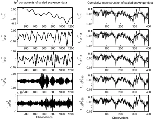
reconstruction. ... 57 Figure 4.20 tpT components of the scaled scavenger data (left column) and cumulative
reconstruction. ... 58 Figure 4.21 One-step ahead prediction of the froth stability in the cleaner for all four modelling strategies. The number supplied in brackets next to each model indicate the correlation of the modelling results with the original time series. ... 59 Figure 4.22 One-step ahead prediction of the froth stability in the rougher for all four modelling strategies. The number supplied in brackets next to each model indicate the correlation of the modelling results with the original time series. ... 59 Figure 4.23 One-step ahead prediction of the froth stability in the scavenger for all four
modelling strategies. The number supplied in brackets next to each model indicate the
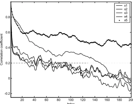
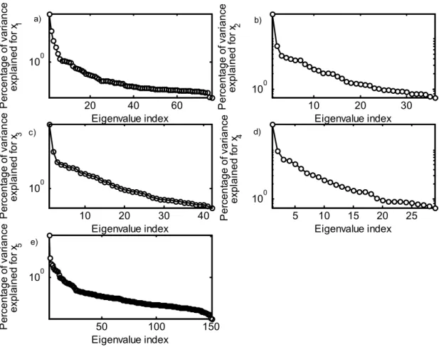
correlation of the modelling results with the original time series. ... 60 Figure 4.24. Measurements of Zn, Pb and Cu in the scavenger circuit collected at 12-minute intervals. ... 61 Figure 4.25 Autocorrelation functions of data from scavenger circuit of base metal flotation plant. ... 62 Figure 4.26 Percentage of variance explained by each eigenvalue for a) Cu, b) Pb and c) Zn time series. ... 63 Figure 4.27 Model predictions of the Cu, Pb and Zn concentrations in the scavenger circuit. Numbers in brackets indicate the fraction of the variance in the original data explained by the model. ... 65 Figure 4.28 (a) Free-run prediction of Zn in the scavenger circuit by use of Model A, and (b) a close-up of the data shown in (a). ... 66 Figure 4.29 Free-run predictions of (a) Cu and (b) Pb concentrations in the scavenger circuit of the base-metal flotation plant. ... 66 Figure 4.30 Autocorrelation function of variables x1 to x5 from lead flotation plant... 67 Figure 4.31 Percentage of variance explained by each eigenvalue and principal component for a) x1, b) x2, c) x3, d) x4 and e) x5 time series... 68
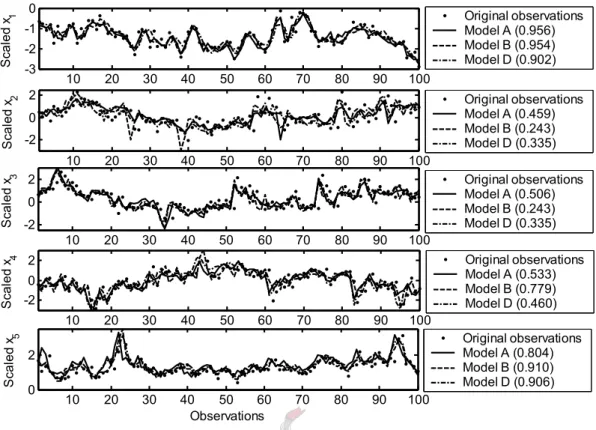
Figure 4.32 Model fits to froth features (x1-x5) with modelling strategies A, B and D. The number supplied in brackets next to each model indicate the correlation of the respective modelling results with the original time series. ... 70
Figure 4.33 Sine wave contaminated by white noise of different variance. ... 71 Figure 4.34 Sine wave contaminated by autocorrelated noise using different values of α... 72 Figure 4.35 Sine wave contaminated by dynamic noise using different variances for the randomly generated error function. ... 72
Figure 5.1 Actual system response (solid line), simulated measured response with nonlinear error (+) and pulsed input signal (broken line) obtained from flow in four tanks in series... 76 Figure 5.2 Autocorrelation function of four tanks in series time series obtained from linear SSA... 77 Figure 5.3 Autocorrelation function of a) part 1, b) part 2, c) part 19 and d) part 20 of four tanks in series time series obtained from localized SSA... 77 Figure 5.4 Percentage of variance explained by eigenvalues of four tank time series analysed by linear SSA. ... 78 Figure 5.5 Percentage of variance explained by eigenvalues of a) part 1, b) part 2, c) part 19 and d) part 20 of the four tank time series analysed by localized SSA. ... 79 Figure 5.6 Section of the reconstructed time series obtained from linear SSA (solid line) and localized SSA (dotted line) compared to the true system dynamics (dotted markers)... 80 Figure 5.7 Individual tpT components of four-tank time series obtained by linear SSA. ... 81
Figure 5.8 Individual tpT components of four-tank time series obtained by localized SSA. .... 82
Figure 5.9 Experimental set-up used to measure electrochemical noise data... 83 Figure 5.10 Enlargement of corrosion cell... 83 Figure 5.11 Original current observations from the electrochemical noise process. ... 84 Figure 5.12 Section of the original current observations from the electrochemical noise
process. ... 85 Figure 5.13 Original voltage observations from the electrochemical noise process. ... 85 Figure 5.14 Section of the original voltage observations from the electrochemical noise process. ... 86 Figure 5.15 Combined reconstruction of first and second principal components of the current time series from the electrochemical noise process, indicating the approximate positions of the break points for the different parts of the time series for localized SSA purposes... 87 Figure 5.16 Autocorrelation function of current time series... 88 Figure 5.17 Eigenvalues of current time series from electrochemical noise observations, extracted by using localized (circles) and linear (square) SSA. ... 89 Figure 5.18 Percentage of variance explained by each eigenvalue obtained from linear SSA of current time series from electrochemical noise process. ... 90 Figure 5.19 Percentage of variance explained by eigenvalue for each part of current time series from electrochemical noise process obtained from localized SSA. ... 91 Figure 5.20 Reconstructed time series obtained by linear SSA (solid line) and localized SSA (dotted line) from original observations (dotted markers) of electrochemical current noise process. ... 92 Figure 5.21 Individual principal component pairs obtained from linear singular spectrum analysis of current data from electrochemical noise process... 93 Figure 5.22 Individual principal component pairs obtained from localized singular spectrum analysis of current data from electrochemical noise process... 93 Figure 5.23 Individual nonlinear principal component pairs obtained from auto-associative neural network analysis of current data from electrochemical noise process... 94
Figure 5.24 First nonlinear principal component extracted from the current series of the electrochemical noise data set by using an auto-associative neural network... 95 Figure 5.25 Second nonlinear principal component extracted from the current series of the electrochemical noise data set by using an auto-associative neural network... 95
Figure 6.1 Classification of stationary time series into different classes. ... 98 Figure 6.2 Illustration of the artificial time series used for benchmarking of the Monte Carlo process. ... 100 Figure 6.3 Frequency distribution of observations in original time series with various
characteristics... 101 Figure 6.4 Frequency distributions of observations from three separate surrogate data sets for each artificial time series by using the AAFT algorithm to generate the surrogate data sets.
... 102 Figure 6.5 Eigenspectra of LGX time series along with confidence bands calculated from surrogates generated by the AAFT algorithm. ... 103 Figure 6.6 Eigenspectra and confidence bands testing if the LGX time series has properties similar to an AR(1) process. ... 103 Figure 6.7 Correlation dimension of the LGX time series (solid line) along with the correlation dimensions of 15 surrogate data sets (broken lines) generated by using the AAFT algorithm.
... 104 Figure 6.8 Eigenspectra of BGX time series along with confidence bands calculated from surrogates generated by the AAFT algorithm. ... 104 Figure 6.9 Eigenspectra and confidence bands testing if the BGX time series has similar properties than an AR(1) process... 105 Figure 6.10 Correlation dimension of the BGX time series (solid line) along with the
correlation dimensions of 15 surrogate data sets (broken lines) generated by using the AAFT algorithm. ... 105 Figure 6.11 Eigenspectra of TGX time series along with confidence bands calculated from surrogates generated by the AAFT algorithm. ... 106 Figure 6.12 Eigenspectra and confidence bands testing if the TGX time series has similar properties than an AR(1) process... 107 Figure 6.13 Correlation dimension of the TGX time series (solid line) along with the correlation dimensions of 15 surrogate data sets (broken lines) generated by using the AAFT algorithm.
... 107 Figure 6.14 Eigenspectra of LUX time series along with confidence bands calculated from surrogates generated by the AAFT algorithm. ... 108 Figure 6.15 Eigenspectra and confidence bands testing if the LUX time series has similar properties than an AR(1) process... 108 Figure 6.16 Correlation dimension of the LUX time series (solid line) along with the correlation dimensions of 15 surrogate data sets (broken lines) generated by using the AAFT algorithm.
... 109 Figure 6.17 Eigenspectra of BUX time series along with confidence bands calculated from surrogates generated by the AAFT algorithm. ... 109 Figure 6.18 Eigenspectra and confidence bands testing if the BUX time series has similar properties than an AR(1) process... 110 Figure 6.19 Correlation dimension of the BUX time series (solid line) along with the correlation dimensions of 15 surrogate data sets (broken lines) generated by using the AAFT algorithm.
Figure 6.20 Eigenspectra of TUX time series along with confidence bands calculated from surrogates generated by the AAFT algorithm. ... 111 Figure 6.21 Eigenspectra and confidence bands testing if the TUX time series has similar properties than an AR(1) process... 112 Figure 6.22 Correlation dimension of the TUX time series (solid line) along with the correlation dimensions of 15 surrogate data sets (broken lines) generated by using the AAFT algorithm.
... 112 Figure 6.23 Eigenspectra of AR(1) time series along with confidence bands calculated from surrogates generated by the AAFT algorithm. ... 113 Figure 6.24 Eigenspectra and confidence bands confirming that the generated AR(1) time series has similar properties than the surrogate AR(1) series. ... 113 Figure 6.25 Correlation dimension of the AR(1) time series (solid line) along with the
correlation dimensions of 15 surrogate data sets (broken lines) generated by using the AAFT algorithm. ... 114 Figure 6.26 Eigenspectra of NonLin time series along with confidence bands calculated from surrogates generated by the AAFT algorithm. ... 114 Figure 6.27 Correlation dimension of the NonLin time series (solid line) along with the
correlation dimensions of 15 surrogate data sets (broken lines) generated by using the AAFT algorithm. ... 115 Figure 6.28 Actual system response (solid line), simulated measured response (+) and pulsed input signal (broken line) obtained from flow in four tanks in series... 116 Figure 6.29 Eigenspectrum generated from complete series of four tanks in series data set, along with the confidence limits of the eigenspectrum obtained from Monte Carlo SSA on surrogate data sets generated by using the AAFT algorithm... 117 Figure 6.30 Attractor of the measured response shown in Figure 6.28, including the transient part of the time series from approximately 0-100 observations. ... 118 Figure 6.31 Dimensionless concentration time series of species A (represented by X) used for the analysis... 119 Figure 6.32 Close-up of a section of the dimensionless concentration time series of species A (represented by X) to illustrate the behaviour of the time series... 119 Figure 6.33 Reconstructed attractor from the first three principal components of the X process state. The percentage of the variance represented by each principal component is supplied in parenthesis next to the appropriate axis. ... 120 Figure 6.34 Eigenvalue distribution and confidence intervals for the eigenspectrum of the X process state of the autocatalytic CSTR reactor. The confidence intervals were calculated by means of surrogate data sets calculated from the AAFT algorithm. ... 121 Figure 6.35 Eigenvalue distribution and confidence intervals for the eigenspectrum of the X process state of the autocatalytic CSTR reactor. The confidence intervals were calculated by means of surrogate data sets calculated from the IAAFT algorithm. ... 121 Figure 6.36 Eigenspectra and confidence bands testing if the autocatalytic CSTR reactor time series has similar properties than an AR(1) process... 122 Figure 6.37 Correlation dimension of the X process state of the autocatalytic CSTR reactor (solid line) along with the correlation dimensions of 15 surrogate data sets (broken lines) generated by using the AAFT algorithm... 122
Figure 7.1 Eigenspectrum of copper time series along with confidence limits of the
eigenspectrum, generated with a) IAAFT and b) AAFT algorithms and c) enlargement of the first principal component with the IAAFT confidence limits. ... 125
Figure 7.2 Eigenspectrum of lead time series along with confidence limits of the
eigenspectrum, generated with a) IAAFT and b) AAFT algorithms and c) enlargement of the first principal component with the IAAFT confidence limits. ... 125 Figure 7.3 Eigenspectrum of zinc time series along with confidence limits of the
eigenspectrum, generated with a) IAAFT and b) AAFT algorithms and c) enlargement of the first principal component with the IAAFT confidence limits. ... 126 Figure 7.4 Nonstationarity of the feed to the flotation plant, showing the principal component scores of the first two weeks (o) and the last two weeks of the feed (+). The percentage of the total variance explained by each principal component is shown in parenthesis in the
appropriate axis label... 127 Figure 7.5 Attractor of copper time series. The percentage of the total variance explained by each principal component is shown in parenthesis in the appropriate axis label... 128 Figure 7.6 Attractor of lead time series. The percentage of the total variance explained by each principal component is shown in parenthesis in the appropriate axis label... 128 Figure 7.7 Attractor of zinc time series. The percentage of the total variance explained by each principal component is shown in parenthesis in the appropriate axis label... 129 Figure 7.8 Q-Q plots of Cu, Pb and Zn feed data versus standard normal... 130 Figure 7.9 Experimental set-up used to investigate avalanching behaviour of various types of particles. ... 133 Figure 7.10 Sections of original time series obtained from avalanching experiments to
illustrate difference in flow behaviour. ... 134 Figure 7.11 Transformed time series obtained from the experiments performed on the various granular substances and used for subsequent analysis. ... 134 Figure 7.12 Individual and cumulative reconstructed components of maize-meal on large plate data series. ... 135 Figure 7.13 Individual and cumulative reconstructed components of maize-meal on large plate data series. ... 136 Figure 7.14 Individual and cumulative reconstructed components of cake flour data series.136 Figure 7.15 Individual and cumulative reconstructed components of maize-meal on large plate data series. ... 137 Figure 7.16 Individual and cumulative reconstructed components of maize-meal on large plate data series. ... 137 Figure 7.17 Eigenvalue spectrum of salt time series along with confidence limits for the eigenvalues calculated from surrogate data generated by the IAAFT algorithm. ... 138 Figure 7.18 Enlarged section of eigenvalue spectrum of salt time series along with confidence limits for the eigenvalues calculated from surrogate data generated by the IAAFT algorithm.
... 139 Figure 7.19 Eigenvalue spectrum of cement time series along with confidence limits for the eigenvalues calculated from surrogate data generated by the IAAFT algorithm. ... 139 Figure 7.20 Enlarged section of eigenvalue spectrum of cement time series along with
confidence limits for the eigenvalues calculated from surrogate data generated by the IAAFT algorithm. ... 140 Figure 7.21 Eigenvalue spectrum of cake flour time series along with confidence limits for the eigenvalues calculated from surrogate data generated by the IAAFT algorithm. ... 140 Figure 7.22 Enlarged section of eigenvalue spectrum of cake flour time series along with confidence limits for the eigenvalues calculated from surrogate data generated by the IAAFT algorithm. ... 141
Figure 7.23 Eigenvalue spectrum of maize-meal on large plate time series along with confidence limits for the eigenvalues calculated from surrogate data generated by the IAAFT algorithm. ... 142 Figure 7.24 Enlarged section of eigenvalue spectrum of maize-meal on large plate time series along with confidence limits for the eigenvalues calculated from surrogate data generated by the IAAFT algorithm... 142 Figure 7.25 Eigenvalue spectrum of maize-meal on small plate time series along with
confidence limits for the eigenvalues calculated from surrogate data generated by the IAAFT algorithm. ... 143 Figure 7.26 Enlarged section of eigenvalue spectrum of maize-meal on small plate time series along with confidence limits for the eigenvalues calculated from surrogate data generated by the IAAFT algorithm... 143 Figure 7.27 Correlation dimension of a) Salt, b) Cement, c) Cake flour, d) Maize-meal on large disc and e) maize-meal on small disc time series, as well as the correlation dimension of 15 surrogate data sets generated by IAAFT algorithm... 145 Figure 7.28 Correlation dimension of a) cold maize-meal and b) warm maize-meal, as well as the correlation dimension of 15 surrogate data sets generated by IAAFT algorithm. ... 146 Figure 7.29 Correlation dimension of a) wet sand and b) dry sand, as well as the correlation dimension of 15 surrogate data sets generated by IAAFT algorithm. ... 146 Figure 7.30 Comparison of slope of correlation dimension curves for different particles by plotting high and low measurements. ... 147 Figure 7.31 Reconstructed attractor for cake flour time series with the amount of variance explained by each principal component supplied in brackets next to the appropriate axis... 148 Figure 7.32 Reconstructed attractor for maize meal on a large plate series with the amount of variance explained by each principal component supplied in brackets next to the appropriate axis. ... 148 Figure 7.33 Reconstructed attractor for maize meal on a small plate series with the amount of variance explained by each principal component supplied in brackets next to the appropriate axis. ... 149 Figure 7.34 Reconstructed attractor for tiling cement time series with the amount of variance explained by each principal component supplied in brackets next to the appropriate axis... 149 Figure 7.35 Reconstructed attractor for salt time series with the amount of variance explained by each principal component supplied in brackets next to the appropriate axis. ... 150
LIST OF
TABLES
Table 4.1 Summary of results obtained from modelling with different strategies (A-D), as well as the autocorrelation function, AC(1), at a lag of one for the two-tank in series data set. Network configurations refer to the number of nodes in the input, hidden and output layers respectively... 45 Table 4.2 Summary of results obtained from modelling with different strategies (A-D), as well as the autocorrelation function, AC(1), at a lag of one for each data set from the copper flotation plant. Network configurations refer to the number of nodes in the input, hidden and output layers respectively ... 60 Table 4.3 Summary of results obtained from modelling with different strategies (A and B), as well as the autocorrelation function, AC(1), at a lag of one for each data set from scavenger circuit of the copper flotation plant. Network configurations refer to the number of nodes in the input, hidden and output layers respectively ... 64 Table 4.4 Summary of results obtained from modelling with different strategies (A-D), as well as the autocorrelation function, AC(1), at a lag of one for each data set from the lead flotation plant. Network configurations refer to the number of nodes in the input, hidden and output layers respectively ... 69 Table 4.5 Summary of results from SSA analysis on simulated sine wave time series
supplying the percentage of the variance in the contaminated signal explained by two retained components, as well as the correlation of the reconstructed series with the clean sine wave.
... 73
Table 6.1 Description of data characteristics of artificial time series used for benchmarking of Monte Carlo SSA ... 98
INTRODUCTION
It is well known that reliable and effective process control, diagnostics of system dynamics, troubleshooting and real-time monitoring of assets are vital for the efficient and competitive operation of any process, with the chemical engineering industry being no exception to this. Current tendencies of companies and plants are to increasingly enlarge their capacities, both to increase their turnover in response to an ever-increasing consumer and customer demand and to enlarge their profit margins by benefiting from the cost savings associated with economy of scale. This enlargement of capacities in their turn implies a number of
adjustments in operating procedures, of which the automation of control programs is quite a prominent one.
Improved control of a process by implementing automated control will not only directly impact factors such as the recovery or extraction grades under variable feed conditions, but will also compensate for operator induced disturbances in the processes thereby optimise the
efficiencies of the process in general. Once the dynamic control of a production process is improved, operators can then dedicate all their attention to more value-added control of other assets.
However, the desired cost savings and improved operation would not necessarily be attained by installing any expensive control system purchased. One should rather ensure that the techniques and methods implemented would be relatively easy to integrate into the process and must be maintainable within the framework of the available engineering resources of the plant.
It is well known that the control of chemical engineering plants and processes is no simple matter, due to a number of factors. These include that
• there are many conflicting and opposing goals to be satisfied • the processes are very often nonlinear and multi-variable in nature
• the dynamics behind the processes tend to be complex, making it harder to understand
• many processes can be described as chaotic in that variables bounce around the set-point chaotically
• fundamental or first principal models are more often than not unavailable for application to mineral processing systems
It is especially this last problem, the lack of fundamental models on which to build control systems, that introduces the need to turn to other methods to aid with the control of mineral processing systems. Due to the nature of processes and the way they are operated, the one commodity that is available in abundance in any mineral processing system is data. A single time series recorded from the output of any dynamical system, be it physical, biological, socio-economic or chemical, is the result of the combination of all the interacting variables in the process. Therefore, in principle, this single record could contain information about the dynamics of all the important variables involved in the process and the evolution of the system under consideration. The idea behind singular spectrum analysis is to exploit this inherent information in the time series and to determine some of the system’s key properties by quantifying specific features of the time series.
The information extracted from the data could then serve as a platform which is used to learn more about the process and to optimize operating conditions, as well as to aid with decisions on the operations management and even the business management levels. The challenge lies therefore in finding the appropriate tools to extract this information from the data and applying this newfound insight then to model-based control systems.
Singular spectrum analysis is a relatively new technique that has been developed initially in the climatology research field, but has since been successfully expanded and applied in a variety of research fields, among which the biosciences, geology, economics and solar
physics are but a few. It appears that the only significant application from which SSA has been absent, is the analysis of data obtained from process plants. However, this absence may be due to oversight, as SSA performs a number of functions that are of direct interest and advantage to the analysis of data from process plants.
The basic idea behind singular spectrum analysis is that it is a tool that embeds either a single or multivariate time series into a higher dimensional matrix, which is then decomposed into a set of base functions or constituent components.
The first major advantage that SSA holds is therefore the decomposition of the time series into the various components that constitute the basis of the time series. These components can be investigated in turn to identify major trends in the data, remove components that can be classified as pure noise and extract oscillatory components present in the data. It is especially this ability of SSA to distinguish noise components from that of trend signals that is of great interest, as that can be applied in the filtering of data, which is desirable for a great number of reasons such as data presentation, modelling and so forth.
By application of SSA to the time series, one’s ability to detect change points is also greatly improved and by using refinements of the technique, it is also possible to characterize the data as being linear or nonlinear, stochastic or deterministic and so forth.
The purpose of SSA is not inherently to identify or build any particular model of the time series investigated. It is rather to provide information on the deterministic and stochastic parts of behaviour in the data, even when the time series is short and noisy (Ormerod and
Campbell, 1997)
All these properties are very desirable in the analysis of time series data obtained specifically from process plants, therefore justifying the application of SSA also in the chemical
engineering and metallurgical processing fields.
The objectives of this study on singular spectrum analysis can be summarized as follows: • To perform a literature survey which investigated the methodology behind singular
spectrum analysis, the available modifications to basic singular spectrum analysis and previous applications of singular spectrum analysis in both other research fields and the engineering industry.
• The application of singular spectrum analysis in the filtering of data and the evaluation of the effectiveness of this filtering by building neural network models on the data. • To explore nonlinear singular spectrum analysis and evaluate the relevance of the
different techniques for nonlinear singular spectrum analysis in application to chemical engineering process systems.
• To explore the practical applications of Monte Carlo singular spectrum analysis in the identification and characterization of time series from process systems.
The rest of this work will be structured along the following topics: Firstly, in chapter 2, a general background on the development of SSA and its application in various research fields by other researchers will be discussed. Due to the concepts behind SSA being largely
unfamiliar in the chemical engineering industry, any technical discussions about the technique or applications thereof, will be left out the literature review in chapter 2, but rather discussed in the methodology in chapter 3. Except for a basic discussion about the SSA technique, the algorithms for a number of advancements, such as multivariate SSA, Monte Carlo SSA and nonlinear SSA will also be described in chapter 3.
The next four chapters will be devoted to various case studies in which different approaches to SSA will be illustrated. The most basic approach is that of chapter 4, where either
univariate or multivariate SSA is applied to a time series in order to remove noise from the series after which the series is subsequently modelled. This will be done for both theoretical case studies and real process data, while comparing the results obtained from various modelling techniques.
The basic approach of chapter 4 leads on to a more complicated scenario in chapter 5, where nonlinear processes and data are being analysed by using two different approaches to nonlinear SSA. Once again the nonlinear application of SSA is applied to both a theoretical, simulated time series and real process data.
The last two chapters, chapters 6 and 7 are both concerned with the characterisation of time series by using Monte Carlo singular spectrum analysis. Chapter 6 is used as a
benchmarking chapter, in that the results obtained from the Monte Carlo SSA are verified with time series with known properties. Once the reliability of the approach has been established, Monte Carlo SSA will be used in chapter 7 to characterise some data obtained from chemical engineering processes.
LITERATURE
REVIEW
Singular spectrum analysis is a relatively new technique, developed from methods that are largely unfamiliar to the engineering and specifically the mineral processing industry. It was decided to refrain from providing a detailed literature review of the technique in this section, since the basic methodology have not yet been explained and consequently a discussion on the development might just serve to confuse the reader. Therefore, beside a brief mention of the origins of SSA and the apparent advantages of SSA compared to other spectral analysis techniques, this section is rather devoted to an investigation into the previous applications of singular spectrum analysis, both in the field of engineering and in other fields of research. A discussion on the development and refinement of singular spectrum analysis as technique will then be given in the appropriate methodology sections in chapter 3.
2.1 Origins of singular spectrum analysis
Singular spectrum analysis was developed simultaneously and independently by Broomhead and King (1986) and Fraedrich (1986). Broomhead and King (1986) applied singular spectrum analysis to the problems of dynamical systems theory and the singular spectrum approach to the method of delays was suggested to remove some of the limitations and ambiguities experienced with the method of delays. In their article they laid the mathematical basis used for singular spectrum analysis by combining PCA or SVD and embedding theorems. They also investigated some preliminary artificial time series to illustrate the advantages of using singular spectrum analysis as a statistical tool for qualitative analysis and for the removal of especially white noise from time series.
Fraedrich (1986) used observed weather and climate variables to provide information for descriptions of the properties of the attractors of these dynamical systems and to obtain an estimate of the smallest number of variables necessary to explain the system dynamics. Further groundbreaking work in the methodological development of the singular spectrum analysis toolkit and substantial research on the possibilities of the technique, was done by Robert Vautard and Michael Ghil. Vautard and Ghil (1989) extended the previous research done by Broomhead and King (1986) and refined certain aspects of the application, which will be discussed in more detail in later sections. After applying SSA to various paleoclimatic time series, they found the technique to be very flexible and incisive. They concluded that, even though SSA is related to ordinary spectral analysis, it is considerably more robust to the nonstationarities that can be found in climatic records.
Vautard et al. (1992) distinguish among three major cases encountered when performing data analysis. The first is where the evolution equations governing the data are known and these equations are relatively insensitive to the initial values of the system. The second type of data analysis occurs when the governing equations are also known, but long-term prediction of the data is impossible due to the sensitivity of the system for the initial values. The last class of data analysis is where the evolution equations for the system are completely unknown and often only noisy measurements of one of the variables in a high-dimensional system are available. It is especially with respect to this last class of data that Vautard et al. (1992) identified the potential of SSA. Even though the work focussed on single-channel SSA, they already saw the possibilities of multi-channel SSA to account for the cross-correlation between several variables that were measured simultaneously. A detailed discussion on the application of multichannel SSA (MSSA) will be given in the methodology section, but for now it will suffice to explain that a number of different variables, all relating to the same
phenomena, are analysed simultaneously by using singular spectrum analysis. The purpose of this is to exploit the relationships between variables reflected in the measured time series.
Two very comprehensive works have recently been written on SSA by Elsner and Tsonis (1996) and by Golyandina et al. (2001). In both these works, the necessary mathematical background is supplied, various approaches to the theory and methodology are discussed and all the possible applications of SSA are investigated. More attention will be given to these works in the methodology section.
2.2 SSA compared to other spectral time series
analysis techniques
It was found that, in principle, most processes can be characterised as a function of
frequency, rather than of time. This frequency is known as either the power spectrum or the spectral density. Very irregular motions, such as noise, will have a smooth and continuous spectrum, as such a process excites all frequencies in a given band. This is contrasted by a pure periodic signal where the series can be described by one specific frequency or a limited number of frequencies (Ghil and Yiou, 1996). The challenge is therefore to determine the underlying power spectrum for real time series which lie somewhere between the two
extremes just mentioned. A number of spectral analysis techniques have been developed and this section will be applied to a very brief description of some of the other techniques that can be used in the place of, or in conjunction with, SSA. Comprehensive comparisons between SSA and other spectral analysis techniques, can be found in (Ghil and Taricco, 1997) and (Ghil and Yiou, 1996).
2.2.1 Fourier analysis
Fourier analysis is similar to singular spectrum analysis, in that it also decomposes the time series into a set of base functions. However, in the case of Fourier analysis, these base functions are a linear combination of selected sine and cosine functions. These base functions are therefore fixed, making it hard to approximate localized disturbances, such as frequency pulses, in the time series, compared to the data-adaptive nature of the SSA base functions, as will be discussed later.
2.2.2 Wavelet analysis
Wavelet analysis is generally used as a basic tool for intermittent, complex and self-similar signals. The technique can be described as a mathematical microscope, in that the emphasis can be placed on a specific part of the time series and local structures and singularities can then be extracted from the small part investigated.
The basis of the technique is to reconstruct either the original time series, or a filtered version of it, by combining a family of wavelet transforms, of which the most common are sine functions convoluted with exponential functions. The wavelet basis used can be adapted to satisfy the specific requirements of the time series investigated.
2.2.3 Maximum Entropy Method (MEM)
The main benefit in using the maximum entropy method is to estimate the line frequencies for a time series that was generated by either a linear autoregressive process or an mth order autoregressive process (Ghil and Yiou, 1996). The technique is performed by calculating one more autocorrelation coefficient from the time series as the order of the autoregressive model (m+1). The spectral density equivalent to the most random or least predictable process with the same autocorrelation coefficients can now be determined. If the time series being investigated is not stationary or close to autoregressive the results from MEM should preferably be verified by cross testing with other techniques. It was found by a number of researchers that the performance of MEM can be greatly improved by first applying SSA to the time series to enhance the signal to noise ratio.
2.2.4 Multi-taper method (MTM)
The estimate of the power spectrum provided by the multi-taper method is nonparametric, in that it does not require a specific, parameter dependent model of the process that had generated the time series (Ghil and Yiou, 1996). A set of tapers is used to reduce the
variance of the spectral estimates. This is done by computing a set of independent estimates of the power spectrum from the pre-multiplication of the data with orthogonal tapers.
The specific advantage of MTM is its ability to detect low-amplitude oscillations in relatively short time series.
2.3 Trends analysis with SSA
Singular spectrum analysis has been successfully applied in a variety of disciplines, of which the most common is paleoclimatology and meteorology, with the biosciences, solar physics, economics and general engineering applications also showing a keen interest in the abilities of SSA. These findings from other research will now be discussed, according to the various fields in which SSA was applied.
2.3.1 Climatology and paleoclimatology
As was mentioned before, this is the area of research in which SSA has received the largest amount of attention, probably because this is also the field in which SSA was first applied to the investigation of time series. Even though these time series are not strictly related to the engineering field, there are many similarities between the natures of climatic and mineral processing time series, in that both time series tend to be relatively short with a noisy behaviour. One can therefore benefit substantially from studying the application of SSA to climatic time records.
The exploration of the effectiveness of analysing paleoclimatic time series by using SSA started simultaneously with the development of SSA in the work done by Michael Ghil and Robert Vautard in Vautard and Ghil (1989). SSA was used to describe the main physical phenomena reflected by the data (such as the periods of various oscillations observed in the data) and it was also used for adaptive spectral filters to remove the dominant oscillations of the system. When SSA was applied to the paleoclimatic time series, it also succeeded in clarifying the noise characteristics of the data. They concluded that SSA verified the need for simple nonlinear models by which the dynamic information contained in existing paleoclimatic records could be extracted and explained.
In some further work (Ghil and Vautard, 1991), SSA was applied to global temperature series with the intention of extracting global warming trends and oscillatory modes from the noise parts. The benefits of using different numbers of eigenvalues in the reconstruction of the time series were illustrated. Due to the success of their previous studies on SSA, the aim of this paper was rather to extract useful information from time series than to prove the validity of SSA. It was assumed that the benefit and relevance of SSA had already been proven. In short succession to the article by Ghil and Vautard (1991), Elsner and Tsonis (1991) published an article also investigating the global temperature record by using SSA. This started an intriguing discussion (Allen et al., 1992b, Allen et al., 1992a, Tsonis and Elsner, 1992) on the results obtained and the conclusions derived from these results. However, the discussion focussed on technical aspects of SSA and will therefore rather be addressed in the methodology section.
Further studies focussing on oscillations in the global climate system were undertaken by Schlesinger and Ramankutty (1994). Instead of just analysing the observed global mean temperature changes, a model is used to simulate these temperature changes and the simulated values are then subtracted from the observed values. SSA was then applied to the detrended data, which revealed new oscillations not previously observed during the SSA performed on non-detrended data by Ghil and Vautard (1991), Elsner and Tsonis (1991) and Allen et al. (1992a). Their conclusion was that, when using SSA, any deterministic trends should first be removed from the data, to allow the first eigenvalues to explain dominant oscillations and not the variance explained by trends in the data.
The next step in the analysis of oscillations in weather patterns was the application of multichannel SSA (Plaut and Vautard, 1994). They used multichannel SSA to identify dynamically relevant space-time patterns and as an adaptive filtering technique. A number of other papers were also written to explore the benefit of SSA in extracting oscillations from climatic time series, or to simply apply the technique and make conclusions on the time series from the oscillations that were extracted. In addition to those papers already mentioned, (Cortijo et al., 1995, Lall and Mann, 1995, Naidu and Malmgren, 1995, Yiou et al., 1995, Yiou et al., 1997, Melice and Rucou, 1998, Evans et al., 1999, Shun and Duffy, 1999, Dean et al., 2002, Pohjola et al., 2002) also applied SSA specifically to
paleoclimatic time series obtained from ice cores, marine microfossils, corals and lakes. In all the studies, SSA was used to divide the time series into trends, oscillations and noise, from which the desired components were identified and extracted. In most of the cases, SSA was used in conjunction with other analysis techniques to verify or clarify the results obtained. In the situation where the results from SSA and other spectral techniques, specifically multitaper spectral analysis (MTM), varied slightly (Lall and Mann, 1995), these differences were
attributed to the different window lengths or smoothing parameters used as well as the fact that SSA is time optimal and MTM frequency optimal. More detailed attention about the different spectral analysis techniques will be given at the end of this chapter. In the work done by Shun and Duffy (1999), attention was also given to multichannel SSA. However, the multichannel SSA was used in conjunction with single channel SSA and no comparison was therefore made about the effectiveness of the two approaches.
As it has been mentioned earlier, a substantial amount of research has been done where singular spectrum analysis was used to investigate time series relating to climatology (Allen and Smith, 1994, Corte-Real et al., 1995, Dettinger et al., 1995, Ghirardelli et al., 1995, Lall and Mann, 1995, Naidu and Malmgren, 1995, Plaut et al., 1995, Allen and Robertson, 1996, Solow and Patwardhan, 1996, Benzi et al., 1997, Zhang et al., 1997, Cook et al., 1998, Corte-Real et al., 1998, Robertson and Mechoso, 1998, Shabalova and Weber, 1998, Stahle et al., 1998, Zhang et al., 1998, Dickey et al., 1999, Elsner et al., 1999, Mo, 1999, Shun and Duffy, 1999, Vautard et al., 1999, Lee and Hang, 2000, Mo, 2000, Paegle et al., 2000, Lee, 2001, Masulli et al., 2001, Mo, 2001, Pederson et al., 2001, Prierto et al., 2001a, Prierto et al., 2001b, Ye, 2001, Ye and Cho, 2001, Yu and Mechoso, 2001, Rodo et al., 2002, Wainer and Venegas, 2002, Baratta et al., 2003, Krepper et al., 2003, Robertson and Mechoso, 2003), and these works are in addition to those works that have already been mentioned in this section. In the majority of these studies either univariate or multivariate (single channel or multichannel) SSA was used as a tool in conjunction with other spectral analysis techniques. The main aim behind the application of the technique was to extract trends or oscillations from the data, which were then related to occurrences in other climatological time series. Some exceptions to the application occurred (Allen and Robertson, 1996) where Monte Carlo SSA was used to distinguish modulated oscillations from red noise and (Masulli et al., 2001) where SSA was used for denoising of the time series to aid with forecasting, but the role that singular spectrum analysis played in most papers was relatively standard and one can only truly benefit from their varying viewpoints if one has the necessary background in climatology and meteorology. Although these works are all of great interest, they will therefore not be discussed in detail, but the interested reader is referred to them.
Benzi et al. (1997) applied SSA to an observed series of minimum and maximum
temperatures and daily cumulative precipitation in the Sardinia region over a 42-year period. They tested the effectiveness of SSA as a technique to characterize the spatial and time frequency dependence of meteorological fields. Benzi et al. (1997) investigated cluster analysis on the local density maxima of principal components. In the meteorological field, the presence of a local high density of points shows that a typical climate exists or that spatial patterns recur. They described a technique developed by Molteni et al. (1990) by which to build homogeneous groups around the local density maxima in the phase space. Their approach included the characterization of seasons by using PCA and the mentioned cluster analysis technique and a spectrum analysis of minimum and maximum temperature fields by using both maximum entropy method and SSA.
Their study confirmed the suitability of SSA for the identification of significant climatological characteristics of a region and recognized that, by synthesizing the whole data set by a few representative components, the relevant characteristics of the signal from the data can be extracted effectively. They succeeded in determining the spatial patterns and time
distributed data. These characteristics were not immediately recognizable from the data itself, but the results proved to be in accordance with the known general behaviour of the Sardinian climate.
Shabalova and Weber (1998) once again focused their research on temperature variability and other paleoclimatic issues. They did however experiment with a novel approach by first subjecting the time series to PCA and then using the spatial principal components as the input channels for the MSSA. The signals in the original time series were then computed by convolving the reconstructed components in PCs with the corresponding spatial modes. A number of independent tests were used to check the consistency of the reconstructed trend components and to identify the quasi-periods. Their results showed that similar results were obtained when the original time series was used directly as input channels and when the principal components were used as the input.
Three further areas of study in the group of publications on climatology that have been mentioned earlier that are worth citing specifically, is that of observing fluctuations in the hurricane frequency (Elsner et al., 1999), obtaining climatic information from tree-ring records (Cook et al., 1998, Stahle et al., 1998, Pederson et al., 2001, Gedalof et al., 2002, Pohjola et al., 2002, D'Arrigo et al., 2003) and observing a link between cholera and climatic changes (Pascual et al., 2000, Rodo et al., 2002).
Researchers used information obtained from tree ring chronologies to identify modes and oscillations in climate variabilities in various regions. (Cook et al., 1998, Stahle et al., 1998, Pederson et al., 2001, Gedalof et al., 2002, Pohjola et al., 2002, D'Arrigo et al., 2003). SSA was applied for the decomposition of the series and it was observed that oscillations that were present in the Southern Oscillation Index could successfully be extracted from the tree ring data (Stahle et al., 1998). An unconventional application of SSA was in (Cook et al., 1998), where SSA was used to examine the stability of observed oscillations. SSA was applied to both the full and truncated reconstructions of the time series. It was found that the principal components from both were in good agreement, indicating a high degree of homogeneity in the reconstruction at the specific periods.
Elsner et al. (1999) launched an investigation into the fluctuations in hurricane frequency in the North Atlantic region. The researchers combined SSA with the maximum entropy method (MEM) to obtain the leading modes of oscillation in the annual hurricane frequency.
In two papers (Pascual et al., 2000, Rodo et al., 2002) researchers investigated the relation between the El Nino-Southern Oscillation (ENSO) and the occurrence of cholera. In the first case study, they used data obtained over 18 years for the number of cholera cases reported each month in conjunction with sea surface temperatures (that provides an index for ENSO) for the same period. SSA was used to decompose both the time series and it was attempted to observe overlapping dominant frequencies between the two data series.
In the second study, two separate periods were studied, but instead of using the sea surface temperature data, the Southern Oscillation index was used to provide information about ENSO. The time series representing the cholera information was the percentage of the people that visited the clinic each month that suffered from cholera. SSA was used to isolate the main interannual variability in the data and also to compare the spectra of the two different periods in time.
A further field of research within the climatology framework that have been applying SSA to a number of time series, is that of measurements of the atmospheric temperature and pressure and hence the atmospheric circulation variability (Allen and Smith, 1994, Plaut and Vautard, 1994, Corte-Real et al., 1995, Zhang et al., 1997, Corte-Real et al., 1998, Ribera et al., 2000, Mo, 2001, Grinsted et al., 2003, Robertson and Mechoso, 2003).
An interesting work was that of Ghil and Yiou (1996) in which they gave a summary of what spectral methods can and cannot do for climatic time series. The work described the connections between time series analysis and nonlinear dynamics. They also focussed on signal-to-noise enhancement and presented some recently developed methods used for spectral analysis. The steps to follow for the various techniques, as well as the benefits and shortcomings of the techniques were illustrated by, once again, using a well known climatic time series. A further discussion of this paper will follow at the end of this chapter.
Another unusual application of SSA in the climatology field was that of Hollingsworth et al. (1997) where SSA, together with autoregressive models, was used to analyse a surface pressure time series from Mars and statistically significant spectral powers were isolated. An annual cycle simulation that corresponded to a low atmospheric dust loading, was performed by using the NASA Ames Mars general circulation model and seasonal variations of storm
zones on Mars were identified. It was found that during certain seasons, localized storm zones occurred in certain areas, with the storm zones shifting into higher latitudes during other seasons. These variations in the storm zones during the seasonal cycle will have important implications for Mars’ regional climate.
It can be seen that SSA has been applied by a great number of researchers to a variety of different time series relating to the meteorological and climatology fields. Even though some individual studies varied, the majority of applications of SSA to climatic time series aimed at extracting relevant trends and oscillations from the data. As it has been mentioned before, this research contains many similarities to process engineering applications, as time series obtained from both the climatology field and engineering processes tend to be relatively short and noisy, making it hard to analyse by using conventional techniques.
2.3.2 Biosciences
Singular spectrum analysis has also been applied with great success in the biological and medical research fields. One of the first studies about the advantages of SSA in the biosciences, and specifically neuroelectrical signals, was done by Mineva and Popivanov (1996). They investigated the identification of single-trial readiness by using a method based on SSA. The time series that was measured was the EEG (electroencephalogram) activity of a patient from a specific time before and until a certain period after a voluntary motor act was performed. This brain activity is known as the readiness potential of the person and indicates the preparation for the voluntary movement. The problem that faced the researchers was that this time series was also characterized as being short and noisy, making the usual techniques unsuitable. The aim of the paper was to extract certain parameters from the single-trail readiness potential and it was found that SSA separated the data records into various
components, by which different dynamical stages of the movement preparatory process could be distinguished. They found that components that were hidden in the raw signal, appeared or disappeared around the onset of the readiness potential and these components were successfully revealed by SSA.
Further research on this subject was done by Popivanov et al. (1998), where they followed a combined linear and nonlinear approach. In this study it was pointed out that previous work done on EEG signal dynamics assumed linear dynamics and therefore used linear methods, such as SSA, while there existed no evidence that this type of analysis fully described the dynamics of the process. They first used two linear methods, namely SSA and time-frequency analysis, based on auto-regressive model coefficients. Four nonlinear techniques were also applied to test whether the linear techniques captured all the dynamics of the time series, and these techniques were point-wise dimension, Kolmogorov entropy, largest Lyapunov
exponent and nonlinear prediction. Their results indicated that the transitions in the dynamics of the EEG activity prior to complicated voluntary activities were detected when using both linear and nonlinear characteristics. This lead to the questions of which approach is more appropriate to detect transitions in the dynamics of mental activity and how the alterations in the dynamical characteristics should be interpreted in the aspect of the mental activities that were involved. They found that due to the nature of mental processes, it was more likely that the nonlinear technique would be appropriate. They concluded that their present results did not provide any evidence that the dynamical changes that were detected reflected the mental activity involved in the voluntary movement preparation and recommended that further complex analysis were performed.
These problems were partly addressed by further research by the same authors in
(Popivanov and Mineva, 1999). They pointed out once again that the majority of physiological signals, such as EEG, blood flow, human gait and ECG are characterized by complex
dynamics, such as nonlinearities and nonstationarities and that it is important to be able to distinguish the characteristics of the process underlying the signal from the properties of the observed time series. Classical methods that could be used to determine possible nonlinear or chaotic dynamics are the correlation dimension, entropy analysis and Lyapunov exponents. However, these methods are not as reliable when only relatively short data series containing stochastic components and nonstationarities are available. They therefore developed several approaches that aim at determining the nonstationarities in the data and testing whether nonlinear dynamics exist.
Work in the field of applying SSA to time series of brain electrical activity was also done by Schreiber (2000). He investigated whether nonlinearity was evident in these time series,