DigitalCommons@USU
DigitalCommons@USU
All Graduate Theses and Dissertations Graduate Studies
5-2013
Enhancement of Random Forests Using Trees with Oblique Splits
Enhancement of Random Forests Using Trees with Oblique Splits
Andrejus Parfionovas Utah State University
Follow this and additional works at: https://digitalcommons.usu.edu/etd Part of the Statistics and Probability Commons
Recommended Citation Recommended Citation
Parfionovas, Andrejus, "Enhancement of Random Forests Using Trees with Oblique Splits" (2013). All Graduate Theses and Dissertations. 1508.
https://digitalcommons.usu.edu/etd/1508
This Dissertation is brought to you for free and open access by the Graduate Studies at
DigitalCommons@USU. It has been accepted for inclusion in All Graduate Theses and Dissertations by an authorized administrator of DigitalCommons@USU. For more information, please contact
USING TREES WITH OBLIQUE SPLITS
by
Andrejus Parfionovas
A dissertation submitted in partial fulfillment of the requirements for the degree
of
DOCTOR OF PHILOSOPHY in
Mathematical Sciences
Approved:
Dr. Adele Cutler Dr. Donald Cooley
Major Professor Committee Member
Dr. Christopher Corcoran Dr. Daniel Coster
Committee Member Committee Member
Dr. J¨urgen Symanzik Dr. Mark R. McLellan
Committee Member Vice President for Research and
Dean of the School of Graduate Studies
UTAH STATE UNIVERSITY Logan, Utah
Copyright ⃝c Andrejus Parfionovas 2013 All Rights Reserved
ABSTRACT
Enhancement of Random Forests Using Trees with Oblique Splits
by
Andrejus Parfionovas, Doctor of Philosophy Utah State University, 2013
Major Professor: Dr. Adele Cutler Department: Mathematics and Statistics
This work presents an enhancement to the classification tree algorithm which forms the basis for Random Forests. Differently from the classical tree-based methods that focus on one variable at a time to separate the observations, the new algorithm performs the search for the best split in two-dimensional space using a linear combi-nation of variables. Besides the classification, the method can be used to determine variables interaction and perform feature extraction. Theoretical investigations and numerical simulations were used to analyze the properties and performance of the new approach. Comparison with other popular classification methods was performed using simulated and real data examples. The algorithm was implemented as an ex-tension package for the statistical computing environment R and made available for free download under the GNU General Public License.
PUBLIC ABSTRACT
Enhancement of Random Forests Using Trees with Oblique Splits
by
Andrejus Parfionovas, Doctor of Philosophy Utah State University, 2013
Statistical classification is widely used in many areas where there is a need to make a data-driven decision, or to classify complicated cases or objects. For instance: disease diagnostics (is a patient sick or healthy, based on the blood test results?); weather forecasting (will there be a storm tomorrow, based on today’s atmospheric pressure, air temperature, and wind velocity?); speech recognition (what was said over the phone, based on the caller’s voice level and articulation); spam detection (can the unsolicited commercial e-mails be identified by their content?); and so on.
Classification trees help to answer such questions by constructing a tree-like structure, where the features of the objects are analyzed consequently one at a time in a step-by-step fashion, e.g.,if a patient is coughing – measure his/her temperature, if the temperature is above 100.4◦F (38.0◦C) – listen to the lungs, if there are crackles
or rattling noises – suspect pneumonia. The classification results become more reliable if the decision is made by aggregating many trees created from randomly sampled data into a Random Forest, similarly to consulting several doctors with different training backgrounds before stating a subtle diagnosis.
In this work the tree classification algorithm was enhanced with the ability to con-sider the objects’ features in pairs,similarly to considering a patient’s body mass index (weight together with height) before diagnosing obesity; or considering a customer’s debt-to-income ratio (income together with debt) before approving him/her for a loan. The trees created with the new method are called oblique, because they separate the objects with oblique lines when looking at the pairwise features plots.
Since the new method is able to focus on pairs of features, it can be used to determine which of the pairs are more useful for classification (chosen more often than others), how the features relate and interact with each other.
This work contains theoretical argumentation for the new method, as well as the detailed description of the classification algorithm, which was implemented in a computer software package (download links are provided). The properties and per-formance of oblique trees were investigated using numerical simulations and real data examples. Comparison with other popular classification methods was also performed.
ACKNOWLEDGMENTS
First, I would like to express gratitude to my major professor, Dr. Adele Cutler, for her help and encouragement in writing this paper, and for setting a personal example of a hardworking scientist.
I would also like to thank other committee members, Drs. Donald Cooley, Daniel Coster, Christopher Corcoran, and J¨urgen Symanzik, for their valuable comments and suggestions.
Many thanks to my family: my cousin Inga Maslova for challenging and support-ing me throughout our coopetition; my sister Natalija; and my parents – Svetlana and Victor, who never stopped believing in me.
CONTENTS Page ABSTRACT . . . . iii PUBLIC ABSTRACT . . . . iv ACKNOWLEDGMENTS . . . . vi LIST OF TABLES . . . . ix LIST OF FIGURES . . . . x
1 INTRODUCTION AND LITERATURE REVIEW . . . . 1
1.1 Classification Problem . . . 1
1.2 Traditional Statistical Approaches . . . 2
1.3 Machine Learning Algorithms . . . 5
1.4 Classification Trees . . . 9
1.5 Dissertation Overview . . . 11
2 CLASSIFICATION TREES WITH OBLIQUE SPLITS . . . . 13
2.1 Theoretical Investigation . . . 14
2.2 Algorithm Description . . . 16
2.3 The Role of the Splitting Criterion . . . 21
3 SOFTWARE DESCRIPTION . . . . 24
3.1 Installation and Loading . . . 24
3.2 Training Function (oblq.tree) . . . 25
3.3 Prediction Function (predict.oblq) . . . 28
3.4 Wrapper Function (get.obl.node) . . . 29
3.5 Dendrogram Plotting Function (plot.oblq) . . . 30
3.6 Usage Example . . . 31
3.7 Disambiguation . . . 33
4 PROPERTIES AND PERFORMANCE . . . . 34
4.1 Simulated Data Examples . . . 34
4.1.1 Orthogonal XOR . . . 36
4.1.2 Diagonal XOR . . . 38
4.1.3 Mixed XOR . . . 40
4.1.4 Banana dataset . . . 42
4.2 Real Data Examples . . . 44
4.2.2 Diabetes . . . 46 4.2.3 Heart Disease . . . 48 4.2.4 Ionosphere . . . 50 4.2.5 Liver Disorder . . . 51 4.2.6 Ecoli . . . 53 4.2.7 Vowels . . . 54 4.3 Performance Summary . . . 56
4.4 Iris Data Structure . . . 57
5 VARIABLE SELECTION AND INTERACTION . . . . 59
5.1 Variable Selection Task . . . 59
5.2 Variable Interaction . . . 61 5.3 Visualization . . . 64 6 SUMMARY . . . . 67 6.1 Conclusions . . . 67 6.2 Further Studies . . . 68 REFERENCES . . . . 69 APPENDICES . . . . 73
APPENDIX A TRAINING FUNCTION CODE . . . 74
APPENDIX B PREDICTION FUNCTION CODE . . . 81
APPENDIX C WRAPPER FUNCTION CODE . . . 83
APPENDIX D CORE ALGORITHM CODE . . . 86
APPENDIX E DENDROGRAM FUNCTION CODE . . . 99
APPENDIX F DISAMBIGUATION EXAMPLE . . . 103
LIST OF TABLES
Table Page
4.1 Averaged misclassification rates for the banana dataset. The top re-sults come from R¨atsch et al. (1998). . . 43 4.2 Averaged misclassification rates for the thyroid dataset. The top
re-sults come from R¨atsch et al. (1998). . . 45 4.3 Averaged misclassification rates for the diabetes dataset. The top
re-sults come from R¨atsch et al. (1998). . . 47 4.4 Averaged misclassification rates for the heart disease dataset. The top
results come from R¨atschet al. (1998). . . 49 4.5 Averaged misclassification rates for the ionosphere dataset. The top
part comes from Breiman (2001). . . 51 4.6 Averaged misclassification rates for the liver dataset. The top part
comes from Breiman (2001). . . 52 4.7 Averaged misclassification rates for the ecoli dataset. The top part
comes from Breiman (2001). . . 54 4.8 Averaged misclassification rates for the vowels dataset. The top part
comes from Breiman (2001). . . 55 4.9 Summary of the performance of different classification methods. . . . 56 5.1 Frequencies for the pairs of non-interacting variables selected by 50
single-node oblique trees. . . 63 5.2 Frequencies for the pairs of variables selected by 150 single-node oblique
LIST OF FIGURES
Figure Page
1.1 Stepwise construction of a tree classifier for Fisher-Anderson’s iris dataset. Observations satisfying the node condition follow the left branch, or right otherwise. . . 10 2.1 Projection of the data points onto the line perpendicular to the linear
separator x2 =mx1+b. . . 17
2.2 Angle θij corresponding to the projection line going through two
ob-servations. . . 18 3.1 An oblique tree dendrogram for Fisher-Anderson’s iris dataset.
Obser-vations satisfying the node condition follow the left branch, or right otherwise. . . 32 4.1 Visualization of data patterns for 2 classes: yi=1 (white) and yi=2
(black). . . 34 4.2 Individual (light) and average (dark) misclassification rates for
orthog-onal XOR data using orthogorthog-onal (-×-) and oblique (-◦-) forests of dif-ferent sizes. . . 36 4.3 Misclassification rates in 100 experiments for orthogonal XOR data
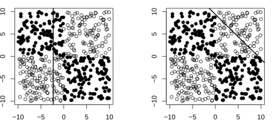
using forests with different numbers of orthogonal (dark) and oblique (white) trees. . . 37 4.4 A typical example of the first splits on XOR data using (a) orthogonal
and (b) oblique separators. . . 38 4.5 Individual (light) and average (dark) misclassification rates for
diago-nal XOR data using orthogodiago-nal (-×-) and oblique (-◦-) forests of dif-ferent sizes. . . 39 4.6 Misclassification rates in 100 experiments for diagonal XOR data using
forests with different numbers of orthogonal (dark) and oblique (white) trees. . . 40
4.7 Individual (light) and average (dark) misclassification rates for mixed XOR data using orthogonal (-×-) and oblique (-◦-) forests of different sizes. . . 41 4.8 Misclassification rates in 100 experiments for mixed XOR data using
forests with different numbers of orthogonal (dark) and oblique (white) trees. . . 41 4.9 A scatterplot of the banana training dataset. Two classes demonstrate
nonlinear structure of the data in two-dimensional space. . . 42 4.10 Pairwise scatterplot of the thyroid dataset (5 variables). . . 46 4.11 Classification of Fisher-Anderson’s iris data using orthogonal tree. . . 57 4.12 Classification of Fisher-Anderson’s Iris data using the oblique tree
clas-sifier. . . 58 5.1 Visualization of the variable importance using the matrix M from the
forest with 50 oblique trees trained on data with: (a) interaction be-tweenx2 and x4, and (b) single variablex2 importance. . . 65
5.2 Visualization of the variable importance from the forest with 500 oblique trees for the ionosphere dataset using (a) the matrix of raw integer scoresM, and (b) the matrix of rescaled observed continuous frequen-cies ln(Oij + 1). . . 66
F.1 Dendrogram for oblique tree trained on Fisher-Anderson’s iris dataset using package obliquetrees version 1.2-1. . . 104 F.2 Dendrogram for oblique tree trained on Fisher-Anderson’s iris dataset
INTRODUCTION AND LITERATURE REVIEW
Statistical classification can be viewed as a part of statistical learning and is widely used for solving pattern recognition, prediction and clustering problems. In this section we describe the general task of classification and different statistical ap-proaches starting with traditional methods, such as discriminant analysis and logistic regression. Next, we will talk about innovative machine learning algorithms: artifi-cial neural networks, adaptive boosting, k-nearest neighbors, support vector machines. Special attention is paid to the tree-based methods such as CART and random forests.
1.1 Classification Problem
Suppose we have a set (population) of objects (observations) that are (or may be) distributed between a number of mutually disjoint classes. We define the problem of classification as a formal task of constructing a rule (algorithm) which learns (trains) using information1 from a given representative sample (training dataset) to assign a class label to an unlabeled observation from the original population. The learning process can be either supervised orunsupervised. The Supervised learning uses train-ing data with labels, which allows to employ all sorts of penalty/reward strategies during the learning process. The Unsupervised learning is looking for a hidden struc-ture in unlabeled data, and is usually referred asclustering orblind signal separation. In this work we will consider classification problems in terms of supervised learning. Different classification algorithms use different approaches, e.g., make different distributional assumptions, use different attributes of the data, etc., which may lead
to different classification results. To verify the performance of a classification method, we use another representative (testing) sample to estimate the probability of misclas-sification. Standard methods of comparison using misclassification rates will allow us to compare the performance of different algorithms applied to different datasets.
Let us now formulate the classification problem using mathematical notation. Suppose there is a set (population) of objects, from which we draw a simple random sample of sizen. Each observation is anm-dimensional vectorxi = (xi1, xi2, . . . , xim)T,
where i = 1,2, . . . , n. We can view xi as a realization of a random variable X =
(X1, X2, . . . , Xm). The class label for each sample observation xi is known (since
this is a supervised learning situation) and denoted by yi, which can be viewed as a
realization of a nominal2 random variable Y, taking values from a set{1,2, . . . , L}. The classification task now is to construct a rule (function or algorithm) that will estimate class the label ˆyj for any unlabeled observation xj from the original
pop-ulation. Definitely, one can come up with many different classification algorithms, say for example, “classify every observation as belonging to class one,” or “classify observations by rolling anL-sided die.” In practice, however, such classifications
tech-niques usually will be of no use. In the next sections we will consider more reasonable classification techniques developed by imposing certain realistic assumptions.
1.2 Traditional Statistical Approaches
Most of the classification methods developed in the statistical community make certain distributional assumptions of the data. We will review the most popular ones.
Linear Discriminant Analysis (LDA) is a classification method that uses a linear combination of features to separate the classes. For simplicity, suppose the observations come only from two classes (L = 2), each with their own multivariate
Gaussian distribution with a common covariance matrix, Σ, and different meansµl: fl(x) = exp{−12(x−µl)TΣ−1(x−µ l) } (2π)m/2|Σ|1/2 , wherex,µl∈Rm, l= 1,2. The prior probabilitiesπ
l for an observation to belong to
class l are estimated by the proportion of class-l observations: nl/n, where n is the
total number of observations in the sample,nl is the number of observations of classl
in the sample. Class labels yi are estimated by ˆyi. Let us denote by P(ˆyi = 2|yi = 1)
the probability of misclassifying the i-th observation as being from class 2 when
it actually comes from class 1. Similarly the probability of misclassifying the i-th
observation to class 1 when it really comes from class 2 is denoted byP( ˆyi = 1|yi = 2).
It then can be shown (Hastie et al., 2001) that the overall misclassification rate
P(ˆyi = 2|yi = 1)π1+P(ˆyi = 1|yi = 2)π2 is minimized when the decision boundary between the two classes is described with a linear discriminant function
δl(x) =xTΣ−1µl− 1 2µ T l Σ− 1µ l+log(πl), l= 1,2.
By equating δ1(x) =δ2(x), the boundary equation can be written as:
(1.1) log ( π1 π2 ) = 1 2 ( µT1Σ−1µ1−µT2Σ−1µ2)−xTΣ−1(µ1 −µ2).
The main drawback of this method is that in practice the normality assumption does not always hold. Even if the normality assumption holds, if the covariance matrices for the groups are different, the linear boundary is not optimal. One must also ensure that the variables used to discriminate between the groups are not highly correlated with each other, otherwise the covariance matrix becomes ill-conditioned and cannot easily be inverted in (1.1).
Logistic Regression (LR) predicts the probability for an object to belong to class l, by applying a logistic function f(x) = (1 +e−x)−1 to a linear combination of
the input variables. Just like for the LDA case, the boundary between classes will be linear. But differently from LDA, the class posterior probabilities are calculated without estimating individual density functions, and thus without requiring the as-sumption of normality. Logistic regression does not assume homogeneity of variances or covariances. However, the log odds (logit) relationship to predictor variables is assumed to be linear: logit(pl(x)) =ln ( pl(x) 1−pl(x) ) =β0+βTx,
where pl(x) = P (Y =l|X =x), l = {1,2}, and parameters β = (β1, β2, . . . , βm)T
andβ0 are estimated from the data. Although originally developed for a dichotomous
output, LR can be generalized for the multiclass case (Hastie et al., 2001). The parameters of the model (β0 and β) are estimated by maximizing the log-likelihood
function: L= n ∑ i=1 ln(pyi(xi)) = n ∑ i=1 [ yi(β0+βTxi)−ln ( 1 + expβ0+βTxi )] .
For a small number of classes, logistic regression is more robust towards the presence of categorical predictors than LDA (Pohar et al., 2004). It also requires fewer assumptions than LDA. However, if the normality assumptions are met, LDA becomes more powerful than LR. One common disadvantage of both methods is that a strong correlation between the input variables may make some of them appear insignificant. Therefore, a proper model selection tool must then be used. An even bigger disadvantage is that both methods use linear boundaries to separate classes, which may not always be appropriate.
1.3 Machine Learning Algorithms
The area of machine learning algorithms is sometimes viewed as a field of arti-ficial intelligence, since its basic idea is to construct a method capable of inductive reasoning, i.e., making a general inference about the population from a premise about a sample (training dataset). The general algorithm usually involves a training (learn-ing) phase, when a model is being fit to the training data, and a testing phase, when the performance of the method is being evaluated on a test dataset. The results ob-tained during the testing phase should not be used for adjusting the model because of the risk of overfitting. For some methods, overfitting may occur during the training phase. To avoid this, the model’s complexity should be controlled and/or the size of the training dataset must be increased.
Below, we describe several widely used machine learning algorithms, which later will be used as the benchmark methods.
k-Nearest Neighbors (k-NN) is a non-parametric classifier which uses the training dataset directly without a training phase. A given observationxi is classified
based on the classes of the k closest points (nearest neighbors), which come from the
training dataset. The majority of the votes of thek nearest neighbors determines the
class label ˆyi, ties are broken at random (Hastie et al., 2001). The main parameter of
the method is the number of nearest neighbors (k), which is chosen arbitrarily. The
distance metric used to determine the closest points does not necessarily need to be Euclidean. This allows the method to be applied to non–numeric variables.
This method is appealing because it makes no assumptions about the data. How-ever, the nearest neighbor rule performs poorly when the number of predictor vari-ables gets large – the so called “curse of dimensionality” (Domeniconi and Gunopulos, 2007). The risk of overfitting and the high computational cost must also be taken into consideration. The computational cost is high mainly because the entire
train-ing dataset must be retained for prediction and distances must be computed to all observations in the training set in order to determine nearest neighbors.
Artificial Neural Networks(ANN) are mathematical models created by simu-lating the topology and functional capabilities of the nervous systems of living organ-isms (i.e., the circuit of biological neutrons of a neural system). The model consists of a number of simple processing elements (neurons) whose behavior is described by a non-linearactivation function of the input arguments (signals). The output of the function might serve as an input for one or more other neurons, thus creating a com-plex structure otherwise known as a neural network (NN). The question of interest is how to find a structure of the network that would be able to model the relationship between the input and output data in a proper way for pattern recognition, discrim-inant analysis, clustering, or classification. Finding a suitable structure of the NN is a nonlinear task of nonlinear optimization with respect to a cost function. The optimization of the NN is done through a training (learning) process using a back-propagation method (Rumelhart et al., 1986). The basic idea is to start with, say, randomly assigned weights of the neurons in the NN, compare the network’s output to the known class (teacher’s output), adjust the neurons’ weights according to the gradient descent learning rule, and keep doing that until the stopping criterion is met (either all observations were classified correctly, or a certain number of iterations was reached).
Some of the drawbacks of NN include a chance of finding local minima (non-optimal solutions), overfitting, and sometimes slow convergence to the solution. The main drawback of the method is its non-robustness: performance highly depends on the structure of the network and the functionality of a single neuron. Thus, for a particular problem it is important to choose a proper topology, cost, and activation function before training the network (Duin, 1996).
Adaptive Boosting(adaBoost) is a general name of an iterative adaptive meta-algorithm which uses an arbitrary weak classifier3 a number of times, each time in-creasing the weights of the misclassified observations and/or dein-creasing the weights of correctly classified ones (Freund and Schapire, 1999). By putting more emphasis on the misclassified observations, the algorithm is adapting to the data structure, which improves the performance. The typical algorithm for a binary classification task (also known as discrete adaBoost) with class labels y∈ {−1,1}, looks as follows:
1. Start with assigning to each observation xi equal weights ω1(i) = 1
n, where i = 1, . . . , n, and n is the sample size. Then for each iteration j repeat the
following steps:
2. Fit a weak classifier of your choice Gj(·) to the data and compute the objective
function (weighted error):
εj = ∑n i=1I{y∑i ̸=Gj(xi)} ·ωj(i) n i=1ωj(i) ,
where I{yi ̸= Gj(xi)} = 1, when yi ̸= Gj(xi), and 0 otherwise (i.e., I is the
indicator function).
3. If εj is small enough (e.g., less than 0.5), then stop. Otherwise, go to the next
step.
4. For each misclassified observation xi update the weight ωj+1(i) =
1−εj
εj
ωj(i)
(leave ωj+1(i) =ωj(i) if it is classified correctly).
5. Go back to step 2.
3The general concept of a weak classifier is that it should perform slightly better than random guessing.
The resultant classifier G∗ is obtained by weighting the weak classifiers Gj selected
during the boosting procedure:
G∗(xi) =sign [ ∑ j Gj(xi)·ln 1−εj εj ] ,
where i= 1,2, . . . , n, and sign means the sign of the expression, i.e. +1 or −1. The modification of the algorithm to fit a real-valued prediction is known asreal adaBoost (Friedman et al., 2000).
The performance of the method highly depends on the choice of the base classifier; overfitting may occur if the weak learner is too complex. It is also sensitive to noise, as it may over-emphasize random fluctuations and perform poorly in later classification (R¨atschet al., 1998).
Support Vector Machines(SVM) were first implemented as a nonlinear gen-eralization of the generalized portrait method by Vapnik and Lerner (1963). The basic idea of the method is to convert the original dataset into a higher dimension to find a separating hyperplane to maximize the distance between the hyperplane and the nearest training datapoints (margin). Later a modification of the method to fit a nonlinear separator was proposed (Boser et al., 1992).
Despite a number of advantages, one of the drawbacks of the method is that it cannot be directly applied for a problem with more than two classes. In this case one has to use either the “one-versus-all” or “one-versus-one” approach: the first separates each one of the labels from the rest, the latter distinguishes between every pair of classes. Both of them, however, have their own shortcomings: the first performs badly when the data are unbalanced, the latter becomes too slow and computationally expensive (Navia-V´azquez, 2007). In the case of a two-class problem SVM may also perform badly if the number of input variables is large, the so called “curse of
dimensionality” (Hastie et al., 2001). The classifier also lacks interpretability.
1.4 Classification Trees
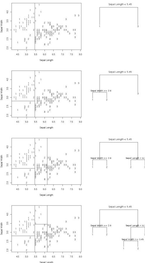
Statistical learning theory defines classification trees as a supervised learning algorithm, which specifies the classification procedure as a set of logical conditions imposed on the input variables. The variables are usually considered one at a time in a sequential order, which allows presentation of the classification in a convenient form of a graph with a tree structure. A step-by-step tree classification procedure is demonstrated in Fig 1.1. The data come from Anderson (1935) and contain 50 records from each of three species (L = 3) of iris flowers.4 The predictor variables
originally include the length and the width of the flowers’ sepals and petals. For simplicity, however, we currently present only two predictors: sepal length and sepal width.
Prediction is based on the values of the predictor variables satisfying the condi-tions at the intermediate nodes of the tree (e.g. xi <0, or xj = 3). The branches of
the tree represent intermediate decisions, which may lead either to another condition (intermediate node), or a conclusion about the values of a class label y (terminal
node) (Hastie et al., 2001). An important feature of such a hierarchical approach
is that each intermediate decision is made using only one variable at a time. This is one of the main differences compared to the classical statistical approaches (such as LR or LDA), which provide us with the decision, considering all the parameters simultaneously.
Also, it is worth mentioning that although the use of heuristic tree-based classi-fication structures dates back to ancient times (e.g. Aristotle’s animal classiclassi-fication system), its comprehensive scientific background remained undeveloped until the end
Fig. 1.1: Stepwise construction of a tree classifier for Fisher-Anderson’s iris dataset. Observations satisfying the node condition follow the left branch, or right otherwise.
of the 20thcentury, when computers became sufficiently powerful to apply the method
for practical purposes. Because of that, tree-based classification techniques have been developing side by side in both statistics [Morgan and Sonquist (1963), Kass (1980), Breiman et al. (1984)] and computer science [Quinlan (1986), Kr¨oger (1996)], which has resulted not only in a different terminology, but also served for applying the methods to quite different problems, such as prediction, feature selection, and data analysis. It is important to keep that in mind, and view each modification of the method in the context of the task it was designed to solve.
Random Forest is a natural development of tree classification, pioneered by Breiman (2001). The basic idea behind the method is to use an ensemble of classifi-cation trees which classify by majority voting. Each tree is fit to a bootstrap sample from the data, a process called bootstrap aggregation (bagging). Instead of finding the best possible split for all m variables, as we would do for a single tree, Random
Forest chooses mtry variables (1≤mtry ≤ m) at random and finds the best split for
them. This is done independently at each node.
It has been shown by Breiman (1996) that in a regression context, using bagging for an unbiased classifier with a high variance (classification tree is one example of such classifier), helps to reduce the prediction variance, without introducing additional bias. In addition to that, Random Forests can be used for estimating the importance of the variables, their relationship (correlation) and interaction, proximity-based clus-tering, etc. It should be mentioned, however, that by being combined in a forest the trees loose their interpretability and become less intuitive.
1.5 Dissertation Overview
This dissertation is organized as follows: Chapter 1 introduces the general ideas of the classification problem, describes traditional and modern classification approaches,
and summarizes their strong and weak points.
In Chapter 2, a new approach is introduced, a theoretical description of its task is presented, and the detailed algorithm of the solution is provided.
The algorithm has been implemented as a set of R functions, which are described in Chapter 3. Instructions on installation and usage are provided. The source code of the functions is attached in the appendices.
Chapter 4 explores the properties and performance of the new method using both simulated and real data examples of different size, dimensionality, and number of classes. The area of applicability of the new method is outlined.
Chapter 5 proposes the application of the new method to the problem of vari-able selection and interaction detection. A way of visualizing information about the variables is suggested.
The conclusions and possible areas for further investigation are summarized in Chapter 6.
Finally, the appendices provide the code of the new algorithm, making it available for other researchers and developers.
CHAPTER 2
CLASSIFICATION TREES WITH OBLIQUE SPLITS
One of the limitations of the classical tree classification techniques is that the de-cisions on splitting the data at each step are made using information only from a single variable at a time. Thus, a single split cannot reflect possible variable interaction, which may be useful in data analysis and/or variable selection. The consideration of variable interaction may also improve the classification performance by making the class separation boundary more flexible to accommodate datasets with a complicated structure. The main goal of this work is to propose a modification for a tree-based classifier, which would consider the interaction between variables by splitting the data in a two-dimensional subspace.
It should be mentioned that the idea of using linear combinations of variables in a tree classifier is not new. In one of the earliest works in this area, Brodley and Utgoff (1992) considered four different ways to navigate through the iterative process of searching the variables’ coefficients to perform a multivariate split. Their meth-ods include: (a) minimization of the mean-squared error over the training dataset (recursive least square algorithm), (b) minimization of the missclassification rate of the training dataset (pocket algorithm), (c) error correction rule which updates the variables’ coefficients so that less attention is paid to large misclassification errors (thermal training), and (d) minimization of the impurity of the multivariate split (CART coefficient learning method). Breiman (2001) introduced the Forest-RC pro-cedure, where the search for the best split is performed over a linear combination of two (or more) randomly selected variables with random coefficients uniformly
dis-tributed on the interval [-1, 1]. Kim and Loh (2001) proposed to use LDA to find the best split among the principal components (linear transformations of variables). Truong (2009) suggested to construct multivariate oblique trees by applying logistic regression to the splits with low values of impurity (ideal splits), which can be iden-tified by performing a number of two-class separations at each node. Another recent approach that follows the path of linear discriminative models to construct splits for multivariate trees was employed by Menzeet al. (2011) usingridge regression at each node.
Differently from the above-mentioned methods, our approach considers all possi-blepairwise combinations of variables at each node. It is also free from the parametric assumptions and attributed drawbacks. Below we present a detailed description of our method.
2.1 Theoretical Investigation
Consider a set ofn points (observations)xi = (xi1, xi2), i= 1,2. . . ninR2 space,
and the appropriate class labels yi ∈ {1,2, . . . , L}. A pair of numbers (m, b) can be
used to construct a linear boundary, x2 = mx1 +b, which separates R2 into two
complementary regions:
R2+mb ={(x1, x2) :mx1+b−x2 ≥0}
and
Each of these regions can be characterized by the proportion of the pointsxibelonging
to different classes, according to yi:
(2.1) pˆ+l = number of {i:xi ∈R 2+ mb AND yi =l} number of {i:xi ∈R2+mb} , l= 1, . . . , L, (2.2) pˆ−l = number of {i:xi ∈R 2− mb AND yi =l} number of {i:xi ∈R2mb−} , l= 1, . . . , L.
Based on that, we define the Gini index as an impurity criterion for each of the regions: (2.3) Gini+= L ∑ l=1 ˆ p+l (1−pˆ+l ), (2.4) Gini−= L ∑ k=1 ˆ p−l (1−pˆ−l ).
The goodness-of-split criterion is defined as a weighted average of the Gini indices (2.3) and (2.4): (2.5) 1 n [ number of {i:xi ∈R2+ab} ·Gini ++ number of{i:x i ∈R2ab−} ·Gini− ] .
The minimization of (2.5) with respect to the pair (m, b), would give us the best
binary linear separator x2 =mx1+b in terms of the split’s impurity. The problem,
however, has no simple analytical solution, and is complicated by local minima, so we minimize (2.5) using an optimized exhaustive search algorithm, described in the following section.
2.2 Algorithm Description
As before, consider an exhaustive search for the best linear separatorx2 =mx1+b
in R2 space for n points x
i = (xi1, xi2), that belong to L classes, where the class of point xi is denoted by yi (i = 1,2, . . . , n). For simplicity, let L = 2 (the case can
be easily extended to a bigger number of classes). Also, suppose no two points are identical, since this leads to an undefined slope of the line going through these points. When such points occur in practice, we add a tiny amount of random noise to separate them.
We are using the fact that in the one-dimensional case, the search for the best binary split using the Gini index as an impurity criterion has been already devel-oped and efficiently implemented in standard tree classification algorithms such as C4.5 (Quinlan, 1993) and CART (Breiman et al., 1984). The original way is quite complicated and proprietary. A simple and relatively efficient way is to move across the sorted values of the variable, updating the values of equations (2.3) and (2.4) as the split moves. Our task then may be considered solved if we manage to show how to reduce the search for a binary split from R2 to R1. To do that, notice that in computing the Gini index for a given binary split one needs no information about the two–dimensional structure of the data in the child nodes.
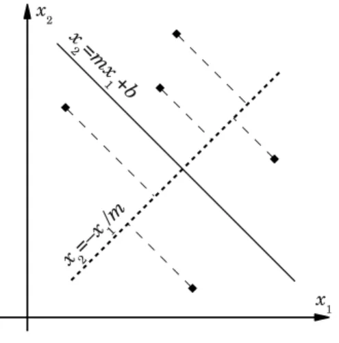
In general, computing the Gini index for a linear separatorx2 =mx1+b requires
knowing of how many data points of each class fall on each side of the separator. This can be easily determined by projecting the data in a direction parallel to the linear separator, i.e., projecting onto a line that is perpendicular to the separator. For separator x2 = mx1 +b we can project onto the line x2 = −xm1 (see Fig. 2.1). Once the data have been projected, the Gini calculation becomes one-dimensional. In fact, this projection allows us to compute the Gini index for any separator that is parallel to x2 = mx1+b, so the best separator in this family can be obtained by
optimizing Gini in the one–dimensional projection. This gives the best separator for the given valuem.
Fig. 2.1: Projection of the data points onto the line perpendicular to the linear separator x2 =mx1+b.
Our goal is to find the best separator over all possible choices of both m and b.
Searching over m involves looking at lines with all possible slopes, i.e., rotating the
line through 180◦. Notice that as the line x2 = mx1 +b rotates, the projected data
points will only give rise to a new Gini index when they change their order. The change of order occurs when two observations (xi1, xi2) and (xj1, xj2) are projected
to the same point. So if we sort the pairs i, j in order of the angleθij they make to
the horizontal (see Fig. 2.2), then one can move through the list of θ’s to determine
which observations will switch positions.
Notice that there is a finite number of linear separators (projection axis x2 =
mx1 +b) that result in different orderings of the data on the line x2 = −xm1. In general, for n points there existn(n−1)/2 possible projection lines unique to within the order of the projected points (number of all possible pairs between then points).
Each ordering may have (n −1) possible splits unique to within the weighted Gini coefficient (2.5). This means that a brute–force exhaustive search for the best split
Fig. 2.2: Angle θij corresponding to the projection line going through two
observa-tions.
amongn points inR2 space requires (n−1)n(n−1)/2 Gini calculations, each of order
O(n), so in general this would be an order O(n4) algorithm.1
In this work, however, we propose an optimization to speed up the search process. Namely, we use the fact that during the process of rotating the projection axis, each new ordering of the projected points differs from the previous one by the order of only two consecutive data points that have been switched. This means that the only new way of splitting the dataset is by putting a split between the points for which the order has been changed. In total, the weighted Gini coefficient (2.5) has to be calculated (n−1) times for the very first vertical projection, and then once for each of the n(n2−1) switched pairs of points. The algorithm can be simplified even more, since every time the order of two points (xi and xj) has being changed, there is no need
to re-calculate Gini from scratch, but only update the values of (2.1) and (2.2) for the appropriate classes (l =yi and l=yj), depending on which points were put from
one side of the split to the other. The complexity of such a Gini update is constant (order O(1)) no matter how many observations there are. This reduces the entire
1The Big-O notation definesf(n) = O(g(n)) if there are positive constantsc and k, such that 0≤f(n)≤cg(n) for alln≥k, wherecand kare fixed for the givenf and must not depend on n
(Knuth, 1976). It is generally used to describe the complexity of an algorithm, e.g., O(n2) means an algorithm should take approximatelyn2 times longer working on an-times bigger dataset.
complexity of the algorithm toO(n2). Also, there is no need to recompute Gini if the
rotation of the projection line switches points from the same class.
The entire algorithm of finding the best linear separator for n points in two–
dimensional space R2 can now be described as follows:2
1. Compute all non-infinite slopes between pairs of data points and arrange them in descending order. If two or more pairs of points have the same slope, we add a tiny amount of random noise to their coordinates to make all slopes unique. This is also used to break ties when ordering observations at step (2) if two or more points have the same x1 coordinate. For further calculations, however,
keep the original coordinates.
2. Make a list of orderings for the observations according to their first coordinate (projection onto thex1axis). For each possible split between consecutive values
ofx1, compute the number of points for each class to the left of the split.3 Save
it for further Gini calculations.
3. Consider a split separating one point on the left and the remainingn−1 points on the right. Compute Gini indices (2.3) and (2.4) for this split and set the appropriate goodness-of-split criterion (2.5) as currently the best.
4. For every other split (with 2,3, . . . ,(n −1) points on the left) compute the goodness-of-split criterion (2.5). If any is smaller than the current best, update the current best and save the coordinates of the corresponding points.
5. Using the list of slopes computed at step (1) choose the pair of points (xi1, xi2)
and (xj1, xj2) with the highest slope. This will be the first pair of points that
2See Appendix C for the C code implementation.
change their order as the projection line starts rotating clockwise from the vertical.
6. Update the list of orderings computed at step (2) for the switched observations. 7. If observations i and j belong to the same class, i.e., yi = yj, go to step (9).
Otherwise, since the observations i and j change their order, the possible split
between them (and only between them) may result in different Gini criteria (2.3) and (2.4). This may affect the goodness-of-split criterion (2.5). To check that, we adjust the number of points that were computed at step (2) for the classesyiandyj to the left of the split (reduce by one for the point that switched
to the right, increase by one for the point that switched to the left).
8. Using the results from the previous step, recompute Gini indices (2.3) and (2.4) considering the split between the switched points (xi1, xi2) and (xj1, xj2).
Find the appropriate goodness-of-split criterion (2.5). If it is smaller than the current best, update the current best and compute the parameters (slope and intercept) of the oblique split line. Slope equals the average of the slope between the current points (xi and xj) and the next largest slope according to the list
from step (1). Intercept equalsxm2−slope·xm1, where xm = (xm1, xm2) is the midpoint between xi and xj. If the split line is vertical, use ∞ as the slope,
and xm1 as the intercept.
9. Repeat steps (6)–(8) for the next largest slope in the list from step (1) until the best goodness-of-split criterion (2.5) is reached.
The algorithm described above is defined for observations in R2. For multidimen-sional datasets we repeat the procedure for all pairs of variables (exhaustive search), or a random subset of pairs. The entire algorithm now looks as follows:
1. Pick two variables (at random, or systematically for an exhaustive search). 2. Find the best split in R2 space to separate classes (see above).
3. Perform steps (1)–(2) for each possible pair of variables (in the case of exhaustive search), or for a smaller, arbitrarily chosen number of times in the case of a random search.
4. After finding the best separating pair of variables, split the dataset and start over at step 1 for each of the descendant nodes, until the nodes are pure. As a result, we obtain a binary decision tree, each node of which tests a condition
xi < mxj +b (xi < b for the vertical lines) to split the data. Since graphically the
separator is generally an oblique line (see Fig. 2.1), we call such splits oblique, in contrast to the classical one-variable splits, which in two-dimensional space would look like lines orthogonal to a chosen variable. Decision trees having oblique splits in the nodes we calloblique trees. Following the concept of the Random Forest, we define oblique forest as an ensemble ofT oblique trees trained on a bootstrap sample from
the training dataset. Once the trees are trained (the forest is grown), the classification of a new observation is performed by majority voting.
2.3 The Role of the Splitting Criterion
As was mentioned in Section 2.1, the Gini impurity measure is used in the oblique tree algorithm as the criterion to make the decision on how to split the dataset at each node. The use of Gini as a splitting criterion has a number of advantages:
Interpretability: Gini has an intuitively simple meaning as a measure of impu-rity: it is minimal when the node is pure (all observations belong to the same class), and is maximal when the node contains equal number of observations from each class.
Computational efficiency: Gini is fast and easy to calculate knowing only the number of points for each class on both sides of the split.
Robustness: Gini is a non-parametric measure which makes no assumptions of the data structure or distribution.
There are, however, certain weaknesses in using Gini as a goodness-of-split cri-terion. The following two seem to influence the classification performance the most.
First of all, even though Gini defines the best split for each particular node, it may not guarantee that the overall solution will be optimal (see the Orthogonal XOR example in Section 4.1). Algorithms that have this property are usually referred to as “greedy” (the terms “myopic” or “short-sighted” are also used sometimes). There are numbers of works aimed to overcome this property by exploring it from different perspectives, to mention a few: Alkhalid et al. (2011) studied 16 different greedy algorithms for decision tree construction (including Gini-based criteria). A dynamic programming based algorithm was used as a reference point for comparison. Murthy and Salzberg (2007) explored the modification of the greedy search with a limited lookahead approach. Kononenko et al. (1997) implemented a system for top-down induction of decision trees using the idea of weighting the variables according to how well they distinguish observations that are “near to each other.” The researches, however, are still facing challenges in this area, e.g. Murthy and Salzberg (2007) have found that “limited lookahead search often produced trees that were worse than the greedy trees in terms of prediction accuracy, tree size as well as depth.” The experimental results of Kononenko et al. (1997) also show that “in the majority of real world problems the myopia has no or only marginal effect.” Nevertheless, the authors consider it “unreasonable to try only myopic algorithm unless it is known in advance that in the dataset there are no strong conditional dependencies between attributes.” Further research, which goes beyond the scope of this work, is definitely
necessary this area.
The other weakness of Gini is the bias towards choosing continuous variables as opposed to categorical variables, as well as towards multilevel categorical vari-ables versus binary ones. This property was first noticed by Breiman et al. (1984): “variables selection is biased in favor of those variables having more values and thus offering more splits” (p. 42). Numbers of attempts to avoid the biased selection have been proposed: Kim and Loh (2001) proposed to use of p-values from association
tests (ANOVA F-test for continuous, and χ2-test for categorical) to select variables
and a bootstrap bias correction. Dobra and Gehrke (2001) usedp-values for the split
criteria under the Null that the distribution of the class label obeys a multinomial distribution. Strobl et al. (2007) derived the exact distribution of the maximally selected Gini gain in the context of binary classification using continuous predictors, and suggested to use the resulting p-values as an unbiased split selection criterion.
Each of the above-mentioned approaches holds their pros and cons, and no universally satisfactory solution has been found yet.
CHAPTER 3
SOFTWARE DESCRIPTION
This chapter describes a set of functions for training and fitting an oblique tree to a given dataset using the R environment for statistical computation and graphics. Instructions on installation and usage are provided. The code for each function is available in the appendices. The source files are also available online.1
3.1 Installation and Loading
Before installing the oblique trees package, the software environment R must be installed.2 The package can be used exactly in the same way on computers with either Microsoft Windows or GNU/Linux (Debian, Redhat, Suse, Ubuntu, etc.) operating systems. The installation process, however, is slightly different. Below we provide step-by-step instructions for either case.
Windows Users:
1. Download the binary archive package.3
2. Start the R software.
3. From the menu “Packages” choose “Install package(s) from local zip files. . .”
4. Locate and open the downloaded file. The rest will be done automatically.
1https://sites.google.com/a/aggiemail.usu.edu/oblique-trees/ 2For download and installation notes visit http://cran.r-project.org/
Linux Users:
1. Download the latest source archive package.4
2. Start the terminal in the directory where you have downloaded the file.
3. Run the following command in the command line prompt using administrative (root) privileges:
R CMD INSTALL obliquetrees_1.2-1.tar.gz
Once the installation is complete, you may start the R software and type:
> library("oliquetrees")
This will load the library for the current session, making the following functions available for use: oblq.tree, predict.oblq, get.obl.node, andplot.oblq. Below we provide the detailed description and usage instructions for these functions.
3.2 Training Function (oblq.tree)
Usage
To grow an oblique tree from the training dataset train.data type:
> oblq.tree(train.data, m.try = 0, min.n = 2, r.seed = 0)
The arguments (parameters)m.try, min.n and r.seed are optional and can be omitted. Their meaning is described below. The value of the function (a data-frame describing the tree) will be returned to the console. To be used for prediction it should be assigned to a variable:
> my.tree <- oblq.tree(train.data)
The code of the function is available in Appendix A.
Arguments
The arguments of the function oblq.tree are defined as follows:
train.data: a matrix or a data frame where the rows correspond to observations and columns representing variables. The last column must contain the class labels (yi). Class labels should be consecutive integer numbers or integer factors i.e.,
1,2, . . . , m. If one or more numbers are omitted, e.g.,{1,4,5}, the program will assume there are 5 classes with classes 2 and 3 having no observations, which may slow down the algorithm performance, since extra memory will be reserved for non-existing classes.
m.try: an optional parameter (integer) which specifies how many possible variable combinations should be tried for each split. The default value 0 will force all possible combinations (m(m2−1), where m is the number of variables). If
m.try̸= 0 then the variables for the splits will be chosen randomlym.trytimes. This might be useful when either the number of variables and/or observations is too large, or when the computer is too slow.
min.n: an optional parameter (integer) which specifies the minimal number of obser-vations that must be in a non-pure node in order for the algorithm to perform a split. The default value is 2. If min.n >2 then a non-pure node with fewer
than min.n points will become terminal, and the class label for it will be set according to the majority of the points. Ties are broken at random. Setting the value of min.n > 2 may help to avoid overfitting when using a single tree
for classification (Khoshgoftaar and Allen, 2001).
r.seed: an optional parameter (integer) which fixes the randomization seed in order to get reproducible results at each run (random numbers are used for breaking ties and separating the overlapping data points). The default value is 0, which
seeds the pseudorandom generator with a current time value to ensure that different numbers are generated each time the program is executed.
Value
The value of the function is a data-frame with the rows corresponding to the nodes of the tree. Each node has the following values:
x, y: the indices of variables on which the split is performed, corresponding to the appropriate columns of the original data train.data.
slope, intercept: the parameters of the node splitting condition:
(3.1) train.data[,x] * slope + intercept > train.data[,y]
when slope<∞, or
(3.2) train.data[,x] < intercept
when slope=∞.
left.node: the row number of the data-frame (child node of the tree) to follow if the observations satisfy the node splitting condition (3.1 or 3.2). If the node is terminal, left.node value is undefined (NA) and the class label for the observations is assigned to left.class.
right.node: the row number of the data-frame (child node of the tree) to follow if the observations do not satisfy the node splitting condition (3.1 or 3.2). If the node is terminal, right.node value is undefined (NA) and the class label for the observations is assigned to right.class.
left.class: the class label to assign for observations that satisfy the condition (3.1 or 3.2) if the node is terminal (NA otherwise).
right.class: the class label to assign for observations that do not satisfy the con-dition (3.1 or 3.2) if the node is terminal (NA otherwise).
3.3 Prediction Function (predict.oblq)
Usage
After an oblique tree my.tree has been grown, it can be applied to the testing dataset test.databy typing:
> predict.oblq(test.data, my.tree)
The value of the function (a vector of predicted values) will be returned to the console. If desired, the value can be assigned to a variable:
> my.prediction <- predict.oblq(test.data, my.tree)
The code of the function is available in Appendix B.
Arguments
The function requires two arguments:
test.data: a matrix with rows corresponding to the observations, and columns rep-resenting the variables. No class labels (yi) are required as opposed to the
training dataset. The columns (variables) must exactly be in the same order as they were in the training matrix.
Value
The value of the function is a vector of class labels for each observation in the testing dataset.
3.4 Wrapper Function (get.obl.node)
Usage
The function get.obl.node is not intended to be used directly by the user. Its purpose is to call an external C function (Appendix D) through the native R interface. It is called internally from the training function (oblq.tree) every time a node of the tree is constructed. The code of the function is available in Appendix C.
Arguments
The function requires four arguments:
max class: the highest value of the class label of the points in the current node (integer). In general it may be smaller than the total number of classes in the entire dataset, but at least as big as the number of different classes in the current node.
x1, x2: two vectors of lengthn of obsrepresenting two variables (selected by the al-gorithm) for the observations in the current node (correspond totrain.data[,x]
and train.data[,y] in the oblq.tree function).
clabels: the class labels of of the observations in the current node.
rand.seed: an optional parameter (integer) which fixes the randomization seed in order to get reproducible results at each run (random numbers are used for breaking ties and choosing the slope of the splitting line). The default value
is 0, which seeds the pseudorandom generator with a current time value to ensure that a different pseudo-random list of numbers is generated each time the program is executed.
Value
The value of the function is a dataset describing the constructed split.
slope, intercept: the parameters of the node splitting condition (3.1 and 3.2).
left.class: the class label to assign for observations that satisfy the node splitting condition 3.1 or 3.2 if the node is pure after splitting.
right.class: the class label to assign for observations that do not satisfy the node condition 3.1 or 3.2 if the node is pure after splitting.
left.Gini: the value of the Gini index for the observations that satisfy the node splitting condition 3.1 or 3.2 if the node is pure after splitting according to 2.4.
right.Gini: the value of the Gini index for the observations that do not satisfy the node condition 3.1 or 3.2 if the node is pure after splitting according to 2.3.
Gini: the weighted Gini index, which is combined from left.Giniand right.Gini
according to 2.5.
3.5 Dendrogram Plotting Function (plot.oblq)
Usage
After an oblique tree my.treehas been grown, it can be visualized as a dendro-gram by typing:
The arguments (parameters) labels.on, main, and cex are optional and can be omitted. Their meaning is described below. The code of the function is available in Appendix E.
Arguments
The arguments of the function plot.oblq are defined as follows:
my.tree: a valid oblique tree data-frame (output of the functionoblq.tree).
labels.on: an optional parameter (boolean), which specifies whether the nodes of the tree should be labeled with their splitting conditions.
main: an optional parameter (text), which is used to set an overall title for the plot. By default the graph will be titled with the my.treeobject’s name.
cex: an optional numeric parameter, which specifies the amount by which labeling text should be scaled relative to the default.
3.6 Usage Example
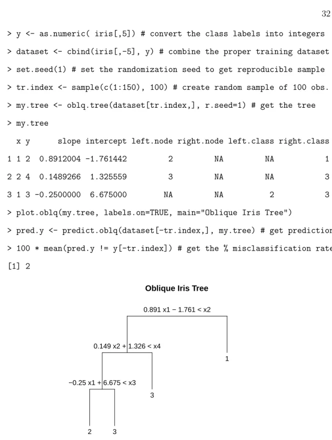
The following example demonstrates the application of the oblique tree classifier to Fisher-Anderson’s iris dataset. Let us generate a training dataset by taking a simple random sample of size 100 without replacement from the original data (150 observations). Use this sample to train an oblique tree and fit it to the remaining 50 observations. The tree dendrogram is presented on Fig. 3.6. Finally, let us compute the percent misclassification rate by comparing the true and predicted values. Below is the corresponding listing of the R program. This code is also available online.5 > library("obliquetrees") # load the package library
> data(iris) # attach the native R dataset
> y <- as.numeric( iris[,5]) # convert the class labels into integers > dataset <- cbind(iris[,-5], y) # combine the proper training dataset > set.seed(1) # set the randomization seed to get reproducible sample > tr.index <- sample(c(1:150), 100) # create random sample of 100 obs. > my.tree <- oblq.tree(dataset[tr.index,], r.seed=1) # get the tree > my.tree
x y slope intercept left.node right.node left.class right.class
1 1 2 0.8912004 -1.761442 2 NA NA 1
2 2 4 0.1489266 1.325559 3 NA NA 3
3 1 3 -0.2500000 6.675000 NA NA 2 3
> plot.oblq(my.tree, labels.on=TRUE, main="Oblique Iris Tree")
> pred.y <- predict.oblq(dataset[-tr.index,], my.tree) # get prediction > 100 * mean(pred.y != y[-tr.index]) # get the % misclassification rate [1] 2
Oblique Iris Tree 0.891 x1 − 1.761 < x2 0.149 x2 + 1.326 < x4 −0.25 x1 + 6.675 < x3 2 3 3 1
Fig. 3.1: An oblique tree dendrogram for Fisher-Anderson’s iris dataset. Observations satisfying the node condition follow the left branch, or right otherwise.
3.7 Disambiguation
The Comprehensive R Archive Network (CRAN) contains a similarly named R package oblique.tree6 by (Truong, 2009) published on June 3, 2009. The package itself and the underlying algorithm of constructing oblique classification trees using logistic regression is different from the one described in this dissertation and was developed independently. The similarity of names is coincidental and purely unin-tentional, as the working draft of the current algorithm and its name was in use long before (Truong, 2009) was published. A simple example (including the appropriate R code) is presented in Appendix F to show the two methods are different. No com-prehensive study of superiority was performed due to the time constrains, since the current work was in the terminal stage by the time we learned about Truong’s work.
CHAPTER 4
PROPERTIES AND PERFORMANCE
In order to explore the performance of classification trees with oblique splits (oblique trees), we have conducted a number of experiments using both simulation and real data examples. Performance of the oblique trees was compared to other widely used statistical classification methods: classical random forests with orthogonal trees, adaBoost, artificial neural network, and support vector machines.
4.1 Simulated Data Examples
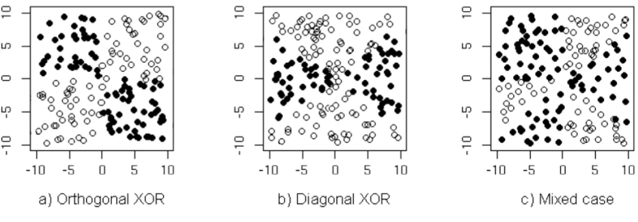
Our first set of experiments is aimed at comparing the performance of random forests when using trees with the classical orthogonal splits versus trees with oblique splits. A simple two–dimensional uniform random variable (X1, X2)∼U[(−10,10)× (−10,10)] was chosen as an input variable. The response variableywas a binary class label, taking values 1 or 2 according to one of the three patterns, so-called orthogonal XOR, diagonal XOR and the mixed XOR case (see Fig. 4.1).
These three patterns were chosen to give some simple, yet non-trivial data struc-tures that could possibly be classified using solely orthogonal (Fig. 4.1a), solely diagonal (Fig. 4.1b), and both orthogonal and diagonal splits (Fig. 4.1c). We used 500 points training dataset to train two ensemble classifiers (forests): one with clas-sical (orthogonal) trees, another with oblique trees. Test dataset (2000 points) was used to compare the performance of the methods by varying the numbers of trees in the forests. The exact steps of the experiment are as follows:
1. Generate the test dataset with 2000 observations. 2. Generate the training dataset with 500 observations. 3. Generate 100 bootstrap samples from the training dataset.
4. Train an orthogonal tree on each of the bootstrap samples from step (3) to get a forest of 100 trees. Classify the test dataset from step (1) using majority voting with 5, 10, 15, . . . , 100 trees, respectively. Compute the misclassification rate. 5. Train an oblique tree on each of the bootstrap samples from step (3) to get a
forest of 100 trees. Classify the test dataset from step (1) using majority voting with 5, 10, . . . , 100 trees, respectively. Compute the misclassification rate. 6. Plot the misclassification rate versus the number of trees (ntr) for both
orthog-onal and oblique forests.
7. Repeat steps (2)–(6) ten times.
8. Compute the average misclassification rate for the forests of different sizes (sep-arately for orthogonal and oblique trees).
Below, we discuss the results of the experiments for each type of data in greater detail. The R code that produces reproducible results using package version 1.0-3 is available in Appendix G. The code is also available online.1
4.1.1 Orthogonal XOR
The class label for the i-th point is defined as yi = 1, if x1ix2i >0, and yi = 2
otherwise (see Fig. 4.1a). One can see that the classes can be perfectly separated using two orthogonal splits along the coordinate axes. Thus, classical trees may have an advantage in this case. The comparison of the misclassification rate for both orthogonal and oblique forests is summarized in Fig. 4.2.
Fig. 4.2: Individual (light) and average (dark) misclassification rates for orthogonal XOR data using orthogonal (-×-) and oblique (-◦-) forests of different sizes.
The forests with orthogonal trees demonstrate consistently smaller misclassifica-tion rates than the forests with oblique trees (0.5% versus 2.5% approximately). The