Types of Strain. Engineering Strain: e = l l o. Shear Strain: γ = a b

Types of Strain

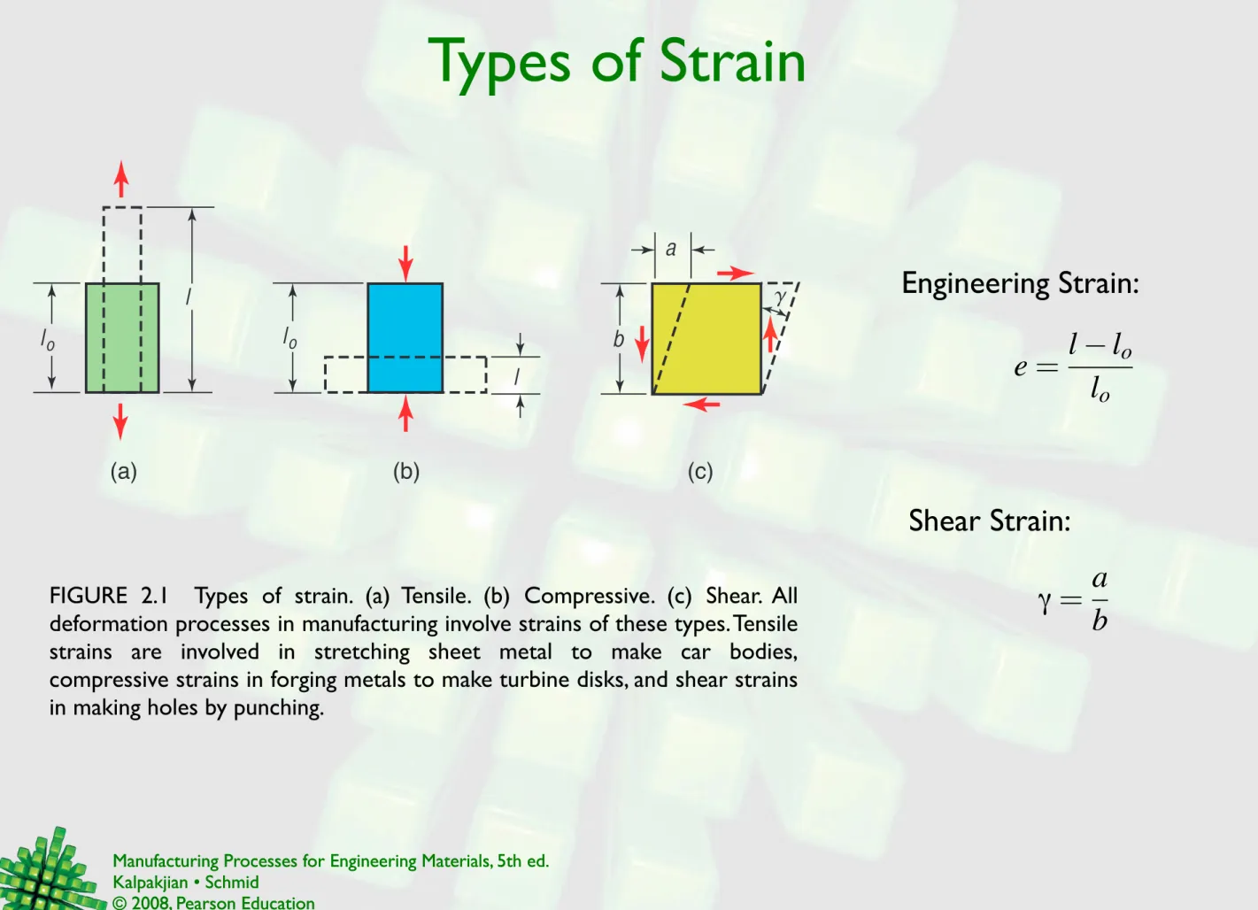
FIGURE 2.1 Types of strain. (a) Tensile. (b) Compressive. (c) Shear. All deformation processes in manufacturing involve strains of these types. Tensile strains are involved in stretching sheet metal to make car bodies, compressive strains in forging metals to make turbine disks, and shear strains in making holes by punching.

(c) (b) (a) l_o l l_o l a b g

e

=

l

−

l

l

γ

=

a

b

Engineering Strain:

Shear Strain:

Tensile-Test

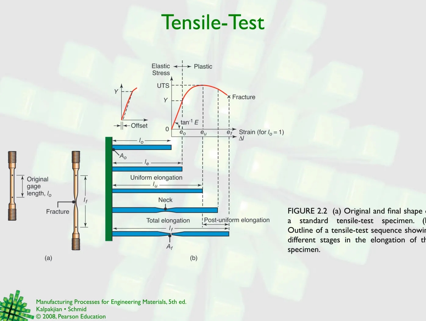
FIGURE 2.2 (a) Original and final shape of a standard tensile-test specimen. (b) Outline of a tensile-test sequence showing different stages in the elongation of the specimen. (a) (b) Original gage length, l_o Fracture l_f tan-1E Plastic Elastic Stress UTS Y Fracture Strain (for l_o = 1) $l e_u e_o e_f 0 Offset A_f A_o Uniform elongation Neck Total elongation Y Post-uniform elongation l_o l_e l_u l_f

Mechanical Properties

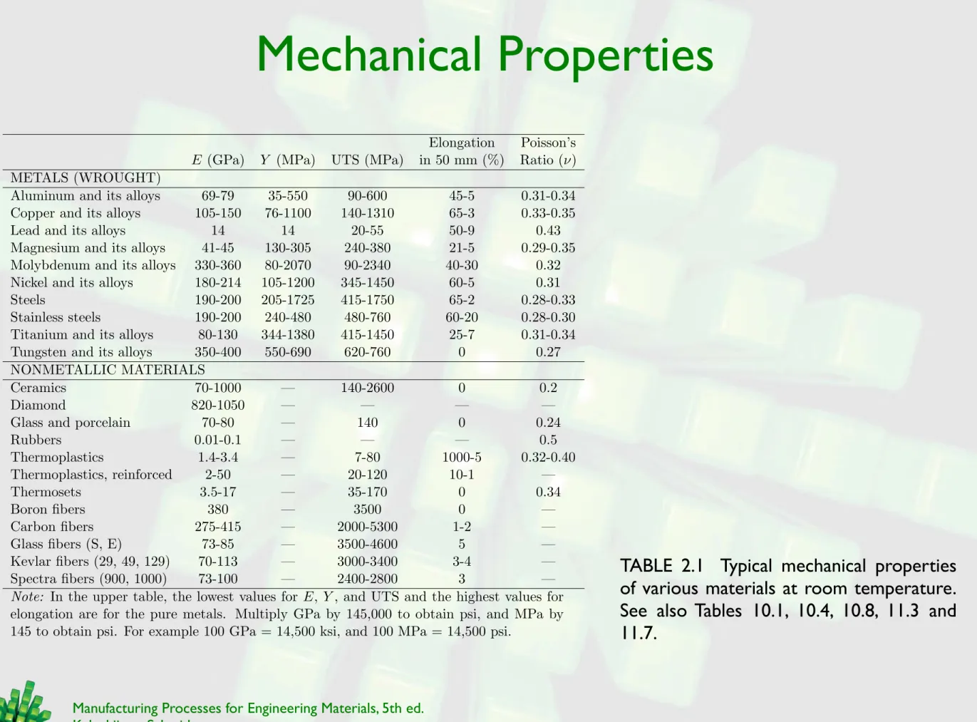
TABLE 2.1 Typical mechanical properties of various materials at room temperature. See also Tables 10.1, 10.4, 10.8, 11.3 and 11.7.

Elongation Poisson’s

E (GPa) Y (MPa) UTS (MPa) in 50 mm (%) Ratio (ν)

METALS (WROUGHT)

Aluminum and its alloys 69-79 35-550 90-600 45-5 0.31-0.34 Copper and its alloys 105-150 76-1100 140-1310 65-3 0.33-0.35

Lead and its alloys 14 14 20-55 50-9 0.43

Magnesium and its alloys 41-45 130-305 240-380 21-5 0.29-0.35 Molybdenum and its alloys 330-360 80-2070 90-2340 40-30 0.32 Nickel and its alloys 180-214 105-1200 345-1450 60-5 0.31

Steels 190-200 205-1725 415-1750 65-2 0.28-0.33

Stainless steels 190-200 240-480 480-760 60-20 0.28-0.30 Titanium and its alloys 80-130 344-1380 415-1450 25-7 0.31-0.34 Tungsten and its alloys 350-400 550-690 620-760 0 0.27 NONMETALLIC MATERIALS

Ceramics 70-1000 — 140-2600 0 0.2

Diamond 820-1050 — — — —

Glass and porcelain 70-80 — 140 0 0.24

Rubbers 0.01-0.1 — — — 0.5 Thermoplastics 1.4-3.4 — 7-80 1000-5 0.32-0.40 Thermoplastics, reinforced 2-50 — 20-120 10-1 — Thermosets 3.5-17 — 35-170 0 0.34 Boron fibers 380 — 3500 0 — Carbon fibers 275-415 — 2000-5300 1-2 — Glass fibers (S, E) 73-85 — 3500-4600 5 — Kevlar fibers (29, 49, 129) 70-113 — 3000-3400 3-4 — Spectra fibers (900, 1000) 73-100 — 2400-2800 3 —

Note: In the upper table, the lowest values for E, Y, and UTS and the highest values for

elongation are for the pure metals. Multiply GPa by 145,000 to obtain psi, and MPa by 145 to obtain psi. For example 100 GPa = 14,500 ksi, and 100 MPa = 14,500 psi.

Loading & Unloading; Elongation

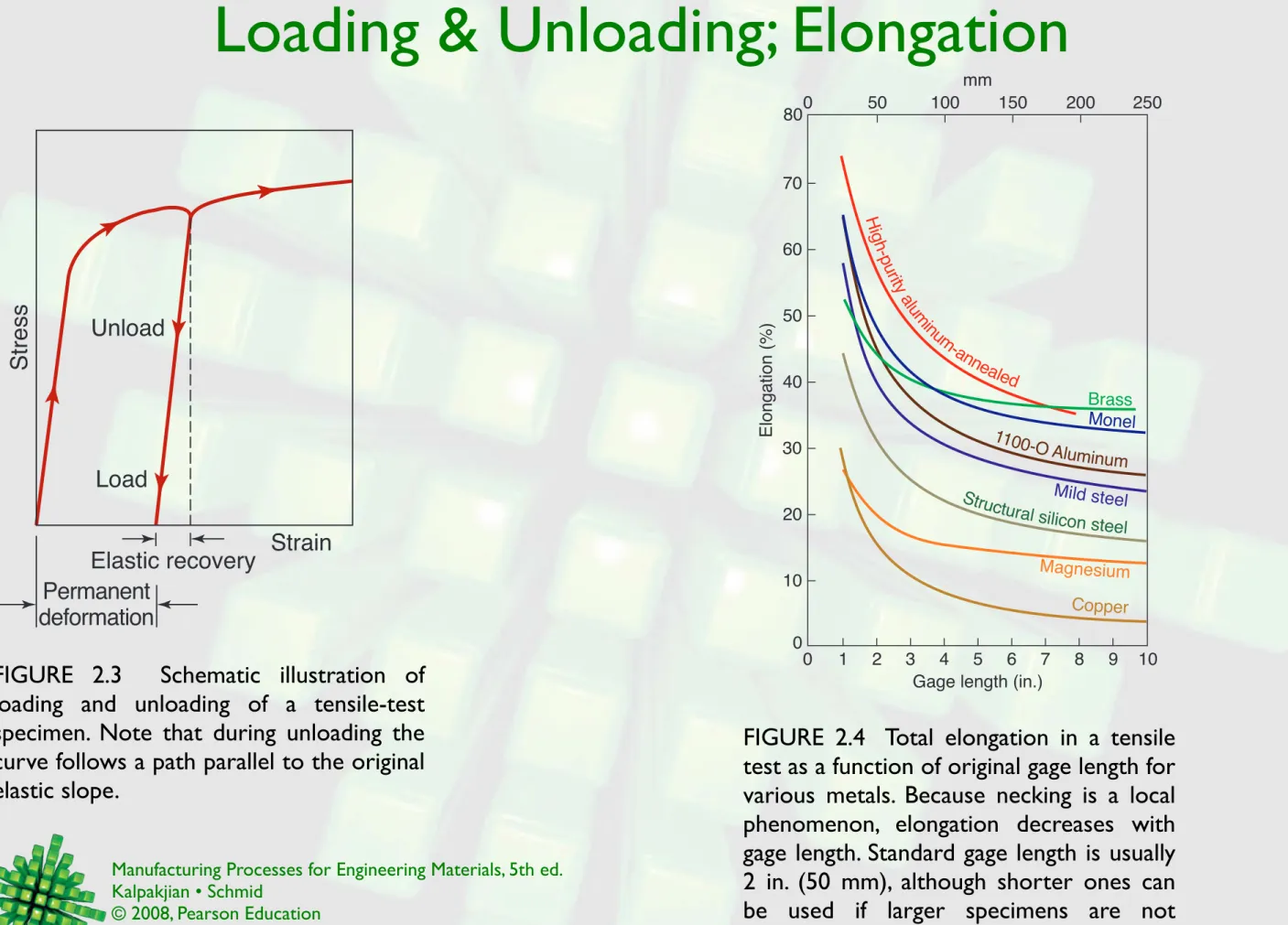
FIGURE 2.3 Schematic illustration of loading and unloading of a tensile-test specimen. Note that during unloading the curve follows a path parallel to the original elastic slope. Elastic recovery Permanent deformation Strain Unload Load Stress

FIGURE 2.4 Total elongation in a tensile test as a function of original gage length for

0 1 2 3 4 5 6 7 8 9 10 80 70 60 50 40 30 20 10 0 0 50 100 150 200 250 Elongation (%)

Gage length (in.) mm

1100-O _Aluminum Mild steel

Structu

ral silicon steel

Magnesium Copper H ig_h -p ur_ity a lu_m inu_m -an neale_d Brass Monel

True Stress and True Strain

TABLE 2.2 Comparison of engineering and true strains in tension

e 0.01 0.05 0.1 0.2 0.5 1 2 5 10 ! 0.01 0.049 0.095 0.18 0.4 0.69 1.1 1.8 2.4

True stress

True strain

σ

=

P

A

ε

=

ln

!

l

l

"

=

ln

!

A

A

"

=

ln

!

D

D

"

=

2 ln

!

D

D

"

True Stress - True Strain Curve

FIGURE 2.5 (a) True stress--true strain curve in tension. Note that, unlike in an engineering stress-strain curve, the slope is always positive and that the slope decreases with increasing strain. Although in the elastic range stress and strain are proportional, the total curve can be approximated by the power expression shown. On this curve, Y is the yield stress and Yf is the flow stress. (b) True

stress-true strain curve plotted on a log-log scale. (c) True stress-true strain curve in tension for 1100-O aluminum plotted on a log-log scale. Note the large difference in the slopes in the elastic and plastic ranges.

True strain (E) T rue stress K Y_f Y 0 0 E₁ 1 E_f S= KEn Fracture (a) n Log E Log S (b) n = 0.25 K = 25,000 0.0001 0.001 0.01 0.1 1 1 10 100 Y

True stress (psi

x 10

3 )

n 1

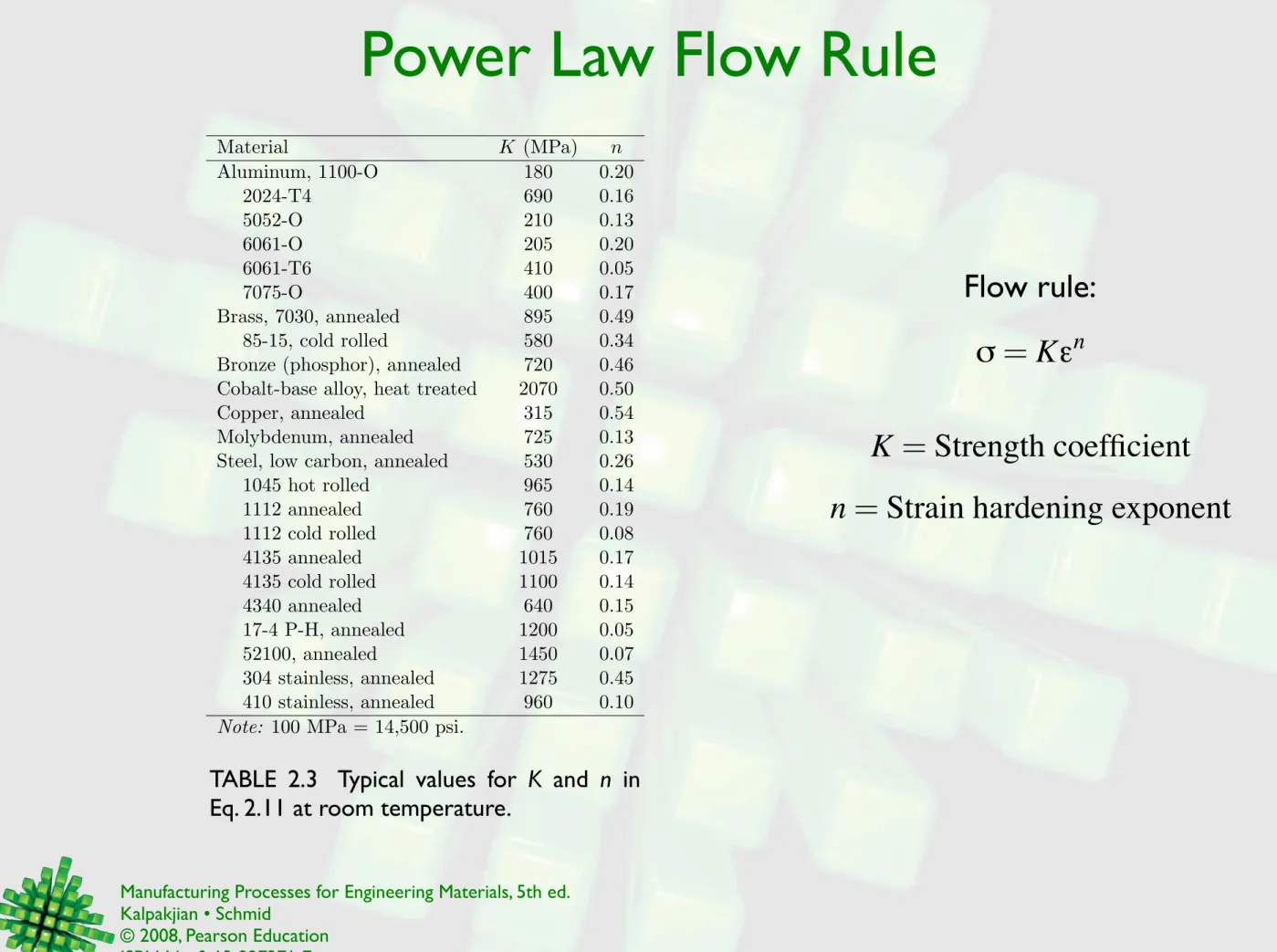
Power Law Flow Rule

TABLE 2.3 Typical values for K and n in Eq. 2.11 at room temperature.

Material K (MPa) n Aluminum, 1100-O 180 0.20 2024-T4 690 0.16 5052-O 210 0.13 6061-O 205 0.20 6061-T6 410 0.05 7075-O 400 0.17 Brass, 7030, annealed 895 0.49 85-15, cold rolled 580 0.34 Bronze (phosphor), annealed 720 0.46 Cobalt-base alloy, heat treated 2070 0.50 Copper, annealed 315 0.54 Molybdenum, annealed 725 0.13 Steel, low carbon, annealed 530 0.26 1045 hot rolled 965 0.14 1112 annealed 760 0.19 1112 cold rolled 760 0.08 4135 annealed 1015 0.17 4135 cold rolled 1100 0.14 4340 annealed 640 0.15 17-4 P-H, annealed 1200 0.05 52100, annealed 1450 0.07 304 stainless, annealed 1275 0.45 410 stainless, annealed 960 0.10

Note: 100 MPa = 14,500 psi.

Flow rule:

σ

=

K

ε

K

=

Strength coefficient

True Stress-True Strain for Various Materials

FIGURE 2.6 True stress-true strain curves in tension at room temperature for various metals. The point of intersection of each curve at the ordinate is the yield stress Y; thus, the elastic portions of the curves are not indicated. When the K and n

values are determined from these curves, they may not agree with those given in Table 2.3 because of the different sources from which they were collected. Source: S. Kalpakjian.

Copper, annealed 2024-T36 Al 0 0.2 0.4 0.6 0.8 1.0 1.2 1.4 1.6 1.8 2.0 0 40 60 80 100 120 140 160 180 1200 1000 800 600 400 0 True strain (E) T

rue stress (psi x 10

3 ) MPa 304 Stainless steel 70–30 Brass, as received 70–30 Brass, annealed 1020 Steel 1100-O Al 1100-H14 Al 6061-O Al 2024-O Al 8650 Steel 1112 CR Steel 4130 Steel 200 20

Idealized Stress-Strain Curves

FIGURE 2.7 Schematic illustration of various types of idealized stress-strain curves. (a) Perfectly elastic. (b) Rigid, perfectly plastic. (c) Elastic, perfectly plastic. (d) Rigid, linearly strain hardening. (e) Elastic, linearly strain hardening. The broken lines and arrows indicate unloading and reloading during the test.

(b) (c) S=Y + Ep! (e) Y S Y + Ep(E -Y/E) Y (d) (a) Y S= Y tan-1 E tan-1 E_p Strain Stress S= EP Y S= Y Y/E S= EE Y/E S EE

FIGURE 2.8 The effect of strain-hardening exponent n on the shape of true stress-true strain curves. When n = 1, the material is elastic, and when n = 0, it is rigid and perfectly plastic.

S = KEn n = 1 0 < n < 1 n = 0 K 0 1 True strain (P) T rue stress

Temperature and Strain Rate Effects

FIGURE 2.9 Effect of temperature on mechanical properties of a carbon steel. Most materials display similar temperature sensitivity for elastic modulus, yield strength, ultimate strength, and ductility.

0 200 400 600 (°C) 0 200 400 600 800 1000 1200 1400 Temperature (°F) Stress (psi 3 10 3 ) 120 80 40 0 Stress (MPa) 600 400 200 0 Elongation Elastic mo_dulus 200 150 100 50 0

Elastic modulus (GPa)

Elongation (%) 0 20 40 60 Tensile strength Yield strength 200 100 50 10 1 2 4 6 8 10 20 30 40 10-6 10-4 10-2 100 102 104 106 Strain rate (s-1)

Tensile strength (psi x 10

3 ) 800 ° 600° 400° 200° 30°C MPa 1000 °

FIGURE 2.10 The effect of strain rate on the ultimate tensile strength of aluminum. Note that as temperature increases, the slope increases. Thus, tensile strength becomes more and more sensitive to strain rate as temperature increases. Source: After J. H. Hollomon.

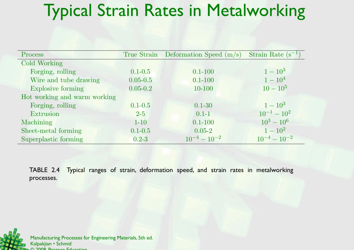
Typical Strain Rates in Metalworking

Process True Strain Deformation Speed (m/s) Strain Rate (s−1₎

Cold Working

Forging, rolling 0.1-0.5 0.1-100 1 ₋ 103

Wire and tube drawing 0.05-0.5 0.1-100 1 ₋ 104

Explosive forming 0.05-0.2 10-100 10 ₋ 105

Hot working and warm working

Forging, rolling 0.1-0.5 0.1-30 1 ₋ 103

Extrusion 2-5 0.1-1 10−1 _{− 10}2

Machining 1-10 0.1-100 103 _{− 10}6

Sheet-metal forming 0.1-0.5 0.05-2 1 ₋ 102

Superplastic forming 0.2-3 10−4 _{− 10−}2 ₁₀₋4 _{− 10−}2

TABLE 2.4 Typical ranges of strain, deformation speed, and strain rates in metalworking processes.

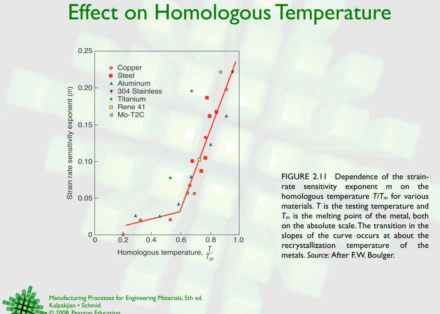
Effect on Homologous Temperature

FIGURE 2.11 Dependence of the strain-rate sensitivity exponent m on the homologous temperature T/Tm for various

materials. T is the testing temperature and

Tm is the melting point of the metal, both

on the absolute scale. The transition in the slopes of the curve occurs at about the recrystallization temperature of the metals. Source: After F. W. Boulger.

0 0.2 0.4 0.6 0.8 1.0 0 0.05 0.10 0.15 0.25 0.20 Copper Steel Aluminum 304 Stainless Titanium Rene 41 Mo-T2C

Strain rate sensitivity exponent (

m

)

T T_m Homologous temperature,

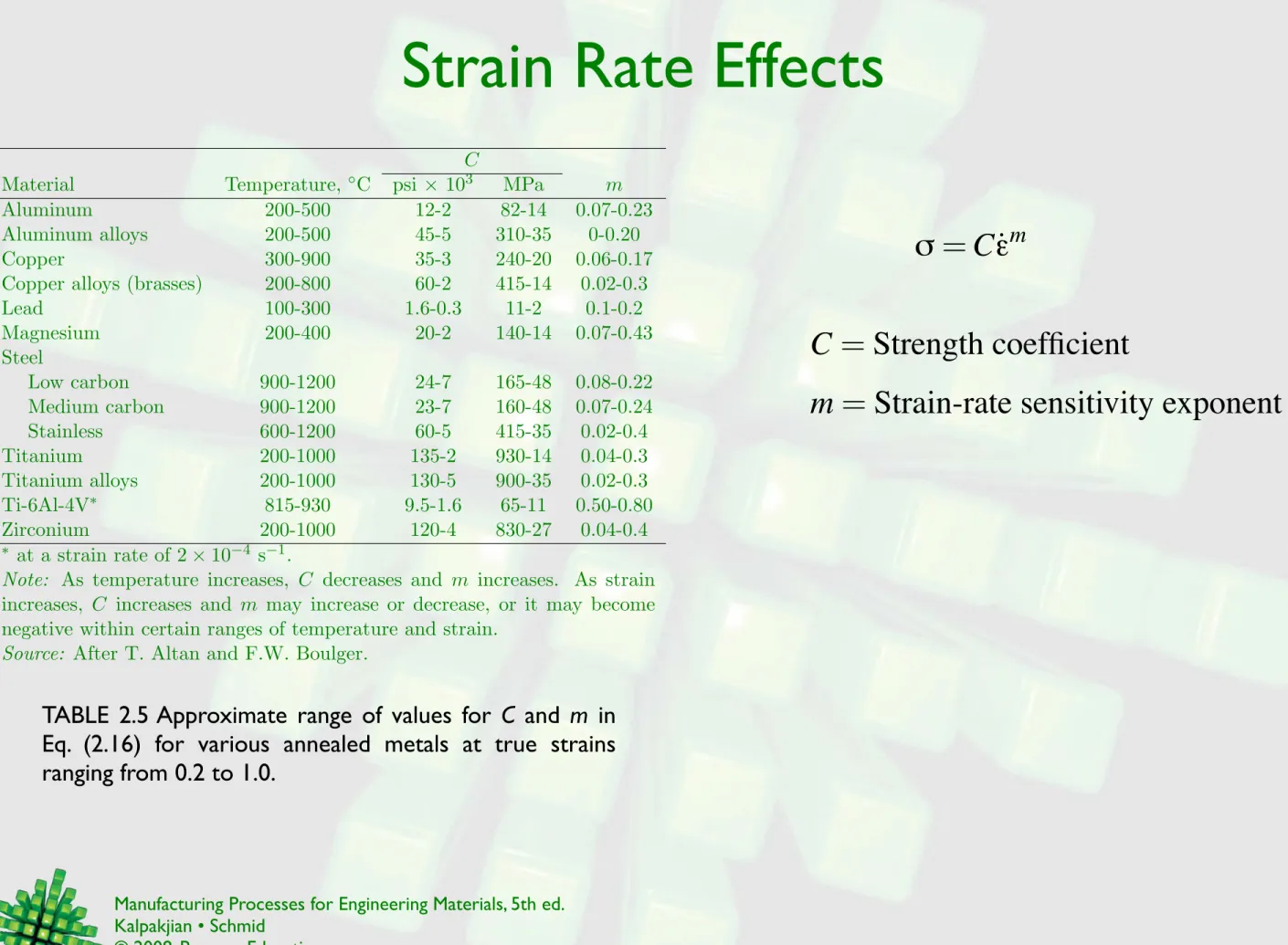
Strain Rate Effects

Material Temperature, ◦_{C psi × 10}3 _{MPa m}

Aluminum 200-500 12-2 82-14 0.07-0.23

Aluminum alloys 200-500 45-5 310-35 0-0.20

Copper 300-900 35-3 240-20 0.06-0.17

Copper alloys (brasses) 200-800 60-2 415-14 0.02-0.3

Lead 100-300 1.6-0.3 11-2 0.1-0.2 Magnesium 200-400 20-2 140-14 0.07-0.43 Steel Low carbon 900-1200 24-7 165-48 0.08-0.22 Medium carbon 900-1200 23-7 160-48 0.07-0.24 Stainless 600-1200 60-5 415-35 0.02-0.4 Titanium 200-1000 135-2 930-14 0.04-0.3 Titanium alloys 200-1000 130-5 900-35 0.02-0.3 Ti-6Al-4V∗ _{815-930 9.5-1.6 65-11 0.50-0.80} Zirconium 200-1000 120-4 830-27 0.04-0.4 ∗ _{at a strain rate of 2×10}−4 _s−1_.

Note: As temperature increases, C decreases and m increases. As strain

increases, C increases and m may increase or decrease, or it may become

negative within certain ranges of temperature and strain.

Source: After T. Altan and F.W. Boulger.

TABLE 2.5 Approximate range of values for C and m in Eq. (2.16) for various annealed metals at true strains ranging from 0.2 to 1.0.

m

=

Strain-rate sensitivity exponent

C

=

Strength coefficient

Effect of Strain Rate Sensitivity on

Elongation

FIGURE 2.12 (a) The effect of strain-rate sensitivity exponent m on the total elongation for various metals. Note that elongation at high values of m approaches 1000%. Source: After D. Lee and W.A. Backofen. (b) The

0.2 0.1 0.3 0.4 0.5 0.6 0.7 0 10 102 103 T otal elongation (%) m Ti–5A1–2.5Sn Ti–6A1–4V Zircaloy–4

High- and ultra-high-carbon steels 0 0.06 0.04 0.02 0 10 30 20 50 40 m Post-uniform elongation (%) A-K Steel HSLA Steel C.R. Aluminum (1100) 2036-T4 Aluminum 3003-O Aluminum 5182-O Aluminum 5182-O Al (150C) 70-30 Brass Zn-Ti Alloy (a) (b)

Hydrostatic Pressure & Barreling

FIGURE 2.13 The effect of hydrostatic pressure on true strain at fracture in tension for various metals. Even cast iron becomes ductile under high pressure.

Source: After H.L.D. Pugh and D. Green.

5 4 3 2 1 0 300 600 900 MPa 0 0 20 40 60 80 100 120 T

rue strain at fracture (

0 f ) Zinc Copper Aluminum Magnesium Cast iron

Hydrostatic pressure (ksi)

FIGURE 2.14 Barreling in compressing a round solid cylindrical specimen (7075-O aluminum) between flat dies. Barreling is caused by friction at the die-specimen interfaces, which retards the free flow of the material. See also Figs.6.1 and 6.2.

Plane-Strain Compression Test

FIGURE 2.15 Schematic illustration of the plane-strain compression test. The dimensional relationships shown should be satisfied for this test to be useful and reproducible. This test gives the yield stress of the material in plane strain, Y’. Source: After A. Nadai and H. Ford.

b

w

h

w

>

5

h

w

>

5

b

b

>

2

h

to

4

h

Yield stress in plane strain:

Y

=

_√

2

Tension & Compression; Baushinger

Effect

FIGURE 2.16 True stress-true strain curve in tension and compression for aluminum. For ductile metals, the curves for tension and compression are identical. Source: After A.H. Cottrell. Tension Compression 0 4 8 12 16 T

rue stress (ksi)

0 0.1 0.2 0.3 0.4 0.5 0.6 0.7 True strain (E) MPa 100 50 0

FIGURE 2.17 Schematic illustration of the Bauschinger effect. Arrows show loading and unloading paths. Note the decrease in the yield stress in compression after the specimen has been subjected to tension. The same result is obtained if compression is applied first, followed by

Y 2Y S P Tension Compression

Disk & Torsion Tests

FIGURE 2.18 Disk test on a brittle material, showing the direction of loading and the fracture path. This test is useful for brittle materials, such as ceramics and carbides. Fracture P P

σ

=

2

P

π

dt

FIGURE 2.19 A typical torsion-test specimen. It is mounted between the two heads of a machine and is twisted. Note the shear deformation of an element in the reduced section. l l rF rF r r t F

τ

=

T

2

π

r

_t

γ

=

r

φ

l

Simple vs. Pure Shear

FIGURE 2.20 Comparison of (a) simple shear and (b) pure shear. Note that simple shear is equivalent to pure shear plus a rotation.

T₃

S

S

S

S

= -

S

G

2

(a)

(b)

Three- and Four-Point Bend-Tests

FIGURE 2.21 Two bend-test methods for brittle materials: (a) three-point bending; (b) four-three-point bending. The shaded areas on the beams represent the bending-moment diagrams, described in texts on the mechanics of solids. Note the region of constant maximum bending moment in (b), whereas the maximum bending moment occurs only at the center of the specimen in (a).

(a)

(b)

Maximum

bending

moment

σ

=

Mc

I

Hardness Tests

FIGURE 2.22 General characteristics of hardness testing methods. The Knoop test is known as a microhardness test because of the light load and small impressions. Source: After H.W. Hayden, W.G. Moffatt, and V. Wulff.

Load, P Hardness number Shape of indentation

Side view Top view Test Indenter 60 kg 150 kg 100 kg 100 kg 60 kg 150 kg 100 kg 500 kg 1500 kg 3000 kg 25 g–5 kg 1–120 kg L 136° HK = 14.2P L2 HV = 1.854P L2 HB = (PD)(D - D2- d2 ) 2P t =mm t = mm 120° L b t L/b = 7.11 b/t = 4.00 d d D = 100 - 500t HRA HRC HRD E Rockwell Knoop Brinell Vickers A C D B F G HRE = 130 - 500t HRB HRF HRG Diamond cone 10-mm steel or tungsten carbide ball Diamond pyramid Diamond pyramid - in. diameter 16 1 steel ball - in. diameter 8 1 steel ball

Hardness Test Considerations

FIGURE 2.23 Indentation geometry for Brinell hardness testing: (a) annealed metal; (b) work-hardened metal. Note the difference in metal flow at the periphery of the impressions.

(a) (b)

d d

FIGURE 2.25 Bulk deformation in mild steel under a spherical indenter. Note that the depth of the deformed zone is about one order of magnitude larger than the depth of indentation. For a hardness test to be valid, the material should be allowed to fully develop this zone. This is why thinner specimens require smaller indentations. Source: Courtesy of

FIGURE 2.24 Relation between Brinell hardness and yield stress for aluminum and steels. For comparison, the Brinell hardness (which is always measured in kg/mm2_{) is converted}

to psi units on the left scale.

Carbon steels, annealed _5.3 1 3.2 3.4 1 1

Aluminum, cold worked

Carbon steels, cold worked MPa 100 200 300 400 500 250 200 150 100 50 0 Hardness (psi x 10 3 ) 10 20 30 40 50 60 70 80 Yield stress (psi x 103)

Brinell hardness (kg/mm 2 ) 150 100 50 0

Fatigue

FIGURE 2.26 Typical S-N curves for two metals. Note that, unlike steel, aluminum does not have an endurance limit.

0 500 400 300 200 100 0 80 60 40 20 1045 Steel Endurance limit Number of cycles, N (a) (b) psi x 1 0 3 Number of cycles, N Stress amplitude, S (MPa) 0 0 2 4 6 psi x 1 0 3 8 10 20 30 40 50 60 Diallyl-phthalate Nylo_{n (d} ry) Po lyc arb onate Po lysu lfone PTFE 103 104 105 106 107 108 109 1010 103 104 105 106 107 20 14 -T6 Alu minu m allo_y Phe nolic Epo_xy Stress amplitude, S (MPa)

FIGURE 2.27 Ratio of fatigue strength to tensile strength

for various metals, as a function of tensile strength. 0.2

0.3 0.4 0.5 0.6 0.7 0.8 0 200 400 600 800 1000 1200 MPa Titanium Steels Cast irons Copper alloys Aluminum alloys Cast

Creep & Impact

FIGURE 2.28 Schematic illustration of a typical creep curve. The linear segment of the curve (constant slope) is useful in designing components for a specific creep life.

Primary Time Tertiary Strain Instantaneous deformation Rupture Secondary Specimen (10 x 10 x 75 mm) Pendulum Pendulum Notch Specimen (10 x 10 x 55 mm) (a) (b)

FIGURE 2.29 Impact test specimens: (a) Charpy; (b) lzod.

Residual Stresses

FIGURE 2.30 Residual stresses developed in bending a beam made of an elastic, strain-hardening material. Note that unloading is equivalent to applying an equal and opposite moment to the part, as shown in (b). Because of nonuniform deformation, most parts made by plastic deformation processes contain residual stresses. Note that the forces and moments due to residual stresses must be internally balanced.

Tensile Compressive (a) (b) (c) (d) a b c o a d o e f

Distortion due to Residual Stress

FIGURE 2.31 Distortion of parts with residual stresses after cutting or slitting: (a) rolled sheet or plate; (b) drawn rod; (c) thin-walled tubing. Because of the presence of residual stresses on the surfaces of parts, a round drill may produce an oval-shaped hole because of relaxation of stresses when a portion is removed.

(c)

(a)

Before

After

Before

After

Before

After

(b)

Elimination of Residual Stresses

FIGURE 2.32 Elimination of residual stresses by stretching. Residual stresses can be also reduced or eliminated by thermal treatments, such as stress relieving or annealing.

Stress (a) (b) Compressive T ensile _S t Sc (c) Y S_t S_c S!_t S!_c Tension Y (d) Compression 2Y

State of Stress in Metalworking

FIGURE 2.33 The state of stress in various metalworking operations. (a) Expansion of a thin-walled spherical shell under internal pressure. (b) Drawing of round rod or wire through a conical die to reduce its diameter; see Section 6.5 (c) Deep drawing of sheet metal with a punch and die to make a cup; see Section 7.6.

(a)

(b)

!

!

!

_!

!

_!

!

!

!

!

!

!

!

!

!

!

Strain State in Necking

FIGURE 2.34 Stress distribution in the necked region of a tension-test specimen.

a Distribution of axial stress Distribution of radial or tangential stress

Maximum axial stress Average axial true stress S = True stress in

uniaxial tension

R 1

2

3

Correction factor due to Bridgman:

σ

σ

=

!

1

1

+

2R

a

"#$

1

+

a

2R

%&

States of Stress

FIGURE 2.35 Examples of states of stress: (a) plane stress in sheet stretching; there are no stresses acting on the surfaces of the sheet. (b) plane stress in compression; there are no stresses acting on the sides of the specimen being compressed. (c) plane strain in tension; the width of the sheet remains constant while being stretched. (d) plane strain in compression (see also Fig. 2.15); the width of the specimen remains constant due to the restraint by the groove. (e) Triaxial tensile stresses acting on an element. (f) Hydrostatic compression of an element. Note also that an element on the cylindrical portion of a thin-walled tube in torsion is in the condition of both plane stress and plane strain (see also Section 2.11.7).

(a) (c) (e) (b) (f) (d) p p p p p p !₁ !₁ !₃ !₁ !₁ !₃ !₂ !₂ !₁ !₃ !₃ !₃ !₃ !₁ !₁ !₃ !₁ !₃

Yield Criteria

FIGURE 2.36 Plane-stress diagrams for maximum

-shear-stress and distortion-energy criteria.

Note that

S

= 0.

Maximum-shear-stress criterion:

Distortion-energy criterion:

σ

−

σ

=

Y

Flow Stress and Work of Deformation

FIGURE 2.37 Schematic illustration of true stress-true strain curve showing yield stress Y, average flow stress, specific energy u1 and flow stress Yf.

Y_f Y Y T rue stress u₁ True strain (!) !₁ 0 0

Flow stress:

Specific energy

¯

Y

=

K

ε

n

+

1

u

=

Z

¯

σ

d

_ε

¯

Ideal & Redundant Work

FIGURE 2.38 Deformation of grid patterns in a workpiece: (a) original pattern; (b) after ideal deformation; (c) after inhomogeneous deformation, requiring redundant work of deformation. Note that (c) is basically (b) with additional shearing, especially at the outer layers. Thus (c) requires greater work of deformation than (b). See also Figs. 6.3 and 6.49.

(a)

(b)

(c)

Total specific energy:

Efficiency:

u

=

u

+

u

+

u

η

=

u