Automated analysis of eclipsing binary light curves - II. Statistical analysis of OGLE LMC eclipsing binaries

Automated analysis of eclipsing binary light curves – II. Statistical

analysis of OGLE LMC eclipsing binaries

T. Mazeh,

O. Tamuz

and P. North

1_{School of Physics and Astronomy, Raymond and Beverly Sackler Faculty of Exact Sciences, Tel Aviv University, Tel Aviv, Israel} 2_{Ecole Polytechnique F´ed´erale de Lausanne (EPFL), Laboratoire d’Astrophysique, Observatoire, CH-1290 Sauverny, Switzerland}

Accepted 2006 January 9. Received 2005 November 30; in original form 2005 September 26

A B S T R A C T

In the first paper of this series, we presented EBAS – Eclipsing Binary Automated Solver, a new fully automated algorithm to analyse the light curves of eclipsing binaries, based on the EBOPcode. Here, we apply the new algorithm to the whole sample of 2580 binaries found in the Optical Gravitational Lensing Experiment (OGLE) Large Magellanic Cloud (LMC) photometric survey and derive the orbital elements for 1931 systems. To obtain the statistical properties of the short-period binaries of the LMC, we construct a well-defined subsample of 938 eclipsing binaries with main-sequence B-type primaries. Correcting for observational selection effects, we derive the distributions of the fractional radii of the two components and their sum, the brightness ratios and the periods of the short-period binaries. Somewhat surprisingly, the results are consistent with a flat distribution in logP between 2 and 10 d. We also estimate the total number of binaries in the LMC with the same characteristics, and not only the eclipsing binaries, to be about 5000. This figure leads us to suggest that (0.7± 0.4) per cent of the main-sequence B-type stars in the LMC are found in binaries with periods shorter than 10 d. This frequency is substantially smaller than the fraction of binaries found by small Galactic radial-velocity surveys of B stars. On the other hand, the binary frequency found byHubble Space Telescope (HST) photometric searches within the late main-sequence stars of 47 Tuc is only slightly higher and still consistent with the frequency we deduced for the B stars in the LMC.

Key words: methods: data analysis – binaries: eclipsing – Magellanic Clouds.

1 I N T R O D U C T I O N

A number of large photometric surveys have recently produced un-precedentedly large sets of high signal-to-noise ratio (S/N) stel-lar light curves (e.g. Alcock et al. 1997). One of these projects is the Optical Gravitational Lensing Experiment (OGLE) study of the Small Magellanic Cloud (SMC) (Udalski et al. 1998) and the Large Magellanic Cloud (LMC) (Udalski et al. 2000), which has already yielded (Wyrzykowski et al. 2003) a few thousand light curves of eclipsing binaries. These two sets of light curves enable a statistical analysis of a large sample of short-period extragalactic binaries, for which the absolute magnitudes of all systems are known to a few per cent. No such sample is known in our Galaxy.

One such statistical study was the analysis of North & Zahn (2003), who derived the orbital elements and stellar parameters of 153 eclipsing binaries discovered by OGLE in the SMC. North & Zahn examined the eccentricities of the eclipsing binaries as a func-tion of the ratio between the stellar radii and the binary separafunc-tion,

_{E-mail: [email protected] (TM); [email protected] (OT)}

and compared their result with a similar dependence derived from the elements of the binaries discovered by Alcock et al. (1997) in the LMC. They then considered the implication of their findings for the theory of tidal circularization of early-type primaries in close binaries (e.g. Zahn 1975, 1977; Zahn & Bouchet 1989).

In a follow-up paper North & Zahn (2004) analysed another set of 510 light curves selected from the 2580 eclipsing binaries dis-covered in the LMC by the OGLE team (Wyrzykowski et al. 2003). Again, they derived the ratio between the stellar radii and the binary separation for these systems, and examined the dependence of the binary eccentricity on this ratio.

The previous analyses used only a small fraction of the sample of eclipsing binaries found in the OGLE data. The goal of the present study is to analyse the whole sample of 2580 light curves discovered by OGLE in the LMC, and to derive some statistical properties of the short-period binaries, after correcting for observational selec-tion effects. Such a correcselec-tion is essential for the derivaselec-tion of the period distribution, for example, because the probability of detect-ing an eclipsdetect-ing binary is a strong function of the orbital period. In order to apply an appropriate correction, one needs a complete homogeneous data set of light curves, all discovered by the same

photometric survey of a well-defined sample of stars. These require-ments were exactly met by the OGLE data set for the LMC, enabling such analysis for a large sample of eclipsing binaries for the first time.

A completely automated algorithm is needed to analyse the large set of eclipsing binaries at hand. Two such codes were developed recently. Wyithe & Wilson (2001) have constructed an automatic scheme based on the Wilson–Devinney (WD) code to analyse the OGLE light curves detected in the SMC in order to find eclips-ing binaries suitable for distance measurements. At the last stages of writing this paper, another study with an automated light curve fitter – Detached Eclipsing Binary Lightcurve (DEBiL) – was pub-lished (Devor 2005). DEBiL was constructed to be quick and simple, and therefore has its own light curve generator, which does not ac-count for stellar deformation and reflection effects. This makes it especially suitable for detached binaries. We will use in this work our EBAS – Eclipsing Binary Automated Solver, which was pre-sented in Paper I (Tamuz, Mazeh & North 2006) and is based on the EBOPcode. The complexity of EBAS is in between DEBiL and the automated WD code of Wyithe & Wilson (2001).

To facilitate the search for global minima in the convolved param-eter space, EBAS performs two paramparam-eter transformations. Instead of the radii of the two stellar components of the binary system, mea-sured in terms of the binary separation, EBAS uses the total radius, which is the sum of the two relative radii, and their ratio. Instead of the inclination, we use the impact parameter – the projected distance between the centres of the two stars in the middle of the primary eclipse, measured in terms of the total radius.

The set of parameters of the EBAS version used here includes the bolometric reflection of the two stars,Ap andAs. WhenAp = 1, the primary star reflects all the light cast on it by the secondary. Together with the tidal distortion of the two components, which is mainly determined by the mass ratio of the two stars, the reflection coefficientsApandAsdetermine the light variability of the system outside the eclipses. Paper I discussed the reliability of the values of these two parameters as found by EBAS.

To simplify the analysis, the present version of EBAS assumes that there is no contribution of light from a third star and that the mass ratio is unity. Paper I discussed the implication of these choices on the values of the parameters, showing that the values of the total radius and the surface brightness ratio are only slightly modified by these two assumptions. The only parameter which is systemati-cally modified by the third-light assumption is the impact parameter, which is directly associated with the orbital inclination of the binary. Note, however, that we are not interested in one specific system but aim, instead, at deriving the gross characteristics of the short-period binaries. As the analysis of this paper does not use the inclinations of the eclipsing binaries for the derivation of the statistical features of the short-period binaries, we regard the resulting distributions as probably correct.

Paper I introduced a new ‘alarm’ statistic,A, to replace human inspection of the residuals. EBAS uses the new statistic, which is sensitive to the correlation between neighbouring residuals to de-cide automatically whether a solution is satisfactory. In this work, we consider only the 1931 systems that yielded solutions with low enough alarm value.

To check the reliability of our results, we compare our geomet-rical elements with those derived by Michalska & Pigulski (2005, hereafter MiP05) with the WD code for 85 binaries, based on the EROS, MACHO and OGLE data. The comparison is reassuring, as it shows that the geometrical parameters of EBAS are close to the ones derived by the more sophisticated WD approach.

To derive the orbital distributions of the short-period binaries, we had to trim the sample, to get a homogeneous sample which we could correct for selection effects. We were left with 938 main-sequence binaries with periods shorter than 10 d and system magnitudes be-tween 17 and 19 in theI band, most of which are binaries with B-type

primaries. This makes the range of the derived period distribution quite narrow. Nevertheless, the data yielded somewhat surprising distributions, which might have implications on binary population studies.

Section 2 presents the resulting orbital elements of the OGLE LMC eclipsing binaries and compares the derived elements with those of MiP05. Section 3 details the procedure to focus on a well-defined homogeneous subsample and Section 4 derives the statistical features of the short-period binaries, after correcting for the obser-vational selection effects. Section 5 discusses the new findings, and Section 6 summarizes this paper.

2 A N A LY S I S O F T H E O G L E L M C E C L I P S I N G B I N A R I E S

The LMC OGLE-II photometric campaign (Udalski et al. 2000) was carried out from 1997 to 2000, during which between 260 and 512 measurements in theI band were taken for 21 fields (Zebrun et al.

2001). Wyrzykowski et al. (2003) searched the photometric data base and identified 2580 binaries. We analysed those systems with EBAS and found 1931 acceptable solutions. Following three types of binaries were excluded.

(i) Four binaries were found to appear twice in the list of bi-naries, with the same period (except for a factor of 2) and with very close positions. Apparently, they originated from the overlap between the different fields of OGLE, and evaded the scrutiny of Wyrzykowski et al. (2003).

(ii) EBAS found 376 solutions with alarm too high –A>0.5. Visual inspection showed that most of these systems are contact binaries thatEBOPcannot model properly. Some might be ellipsoidal variables (see Wyrzykowski et al. 2003) or other types of periodic variables, other than eclipsing binaries.

(iii) EBAS found 269 solutions that yielded sum of radiirt=

rp+rstoo large. Following the Roche lobe radius calculation in Eggleton (1983):

RRL/a=

0.49q2/3

0.6q2/3_+ln(1+q1/3₎, (1) which reduces forq = 1 to RRL/a =0.379, we did not accept solutions with

rt>0.65 (1−e cosω), (2) assuming theEBOPmodel cannot properly account for the deforma-tion of the two stars if one or two stars are too close to their Roche lobe limit, at least at the periastron passage.

We were thus left with 1931 acceptable solutions. 2.1 Solution examples

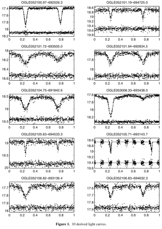
In Fig. 1, we plot 10 representative light curves derived by the EBAS. Their elements are given in Tables 1 and 2. Table 1 gives some global information on each light curve and the goodness-of-fit of its model. It lists the number of measurements, the averaged observedI

mag-nitude and the rms of the scatter of the OGLE light curve. It also lists theχ2_{, the alarmAof the fit and the detectability measureD} (see below), and whether this binary was included in the trimmed sample (+), as detailed in the next section. Table 2 lists the derived

0 0.2 0.4 0.6 0.8 1 17.4 17.6 17.8 18 18.2 OGLE052100.97–692526.3 0 0.2 0.4 0.6 0.8 1 18.6 18.8 19 19.2 19.4 19.6 19.8 OGLE052101.19–694725.0 0 0.2 0.4 0.6 0.8 1 18 18.2 18.4 18.6 OGLE052101.72–693505.0 0 0.2 0.4 0.6 0.8 1 17.8 18 18.2 OGLE052101.94–692834.5 0 0.2 0.4 0.6 0.8 1 18.5 19 19.5 OGLE052104.75–691842.6 0 0.2 0.4 0.6 0.8 1 17.6 17.8 18 18.2 OGLE053008.33–693438.0 0 0.2 0.4 0.6 0.8 1 19 19.5 20 OGLE052105.63–694533.3 0 0.2 0.4 0.6 0.8 1 18.6 18.8 19 19.2 19.4 19.6 OGLE052105.71–693143.7 0 0.2 0.4 0.6 0.8 1 17.7 17.8 17.9 18 OGLE052106.82–693136.4 0 0.2 0.4 0.6 0.8 1 17.6 17.7 17.8 17.9 OGLE052106.83–694632.3

Figure 1. 10 derived light curves.

elements of EBAS and their estimated uncertainties. This includes theI magnitude of the system at quadrature [the luminosity scaling

factor (SFACT) parameter ofEBOP, see table 2 of Paper I], the pe-riod,P, in days, the sum of radii, rt, the ratio of radii,k, the surface brightness ratio,Js, the impact parameter,x, and the eccentricity e, multiplied by cosωand sinω, whereωis the longitude of perias-tron. Note that the mag parameter in Table 2 is the brightness of the system out of eclipse, and therefore is different from the ob-served averaged mag given in Table 1. Since its formal error is very small, we give it to four or five decimal figures because this might be useful for comparison purposes, even though we are well aware that systematic errors – whether in the original photometric data or in their fit – are far larger than that level of accuracy. Let us re-call that some parameters were held fixed in the fit, as explained in Paper I: the linear limb-darkening coefficients, with a value typical

of main-sequence B stars (up=us=0.18), the gravity-darkening coefficients (yp = ys = 0.36), the mass ratio (q =1), the tidal lead/lag angle (t=0) and the third light (L3=0).ApandAsare the bolometric reflection coefficients, the value of which is between 0 and 1; they determine (together with the tidal distortion of the com-ponents) the out-of-eclipse variability. They are adjusted in order to fit the variation outside eclipses, but since reflection effects are only crudely modelled byEBOP, one has to keep in mind that their value may have very limited physical significance.

Of the 10 stars, the light curve of OGLE 052101.72−693505 yieldedrttoo high, and the primary of OGLE 052106.82−693136.4 is probably not a main-sequence star (see below). Therefore, both the stars were not included in the final statistical analysis. Because the system 053008.33−693438.0 has a very shallow secondary min-imum, its ratio of radii is poorly constrained, and it probably has

Table 1. The 10 binaries: observations and goodness-of-fit.

OGLE name N mag rms χ2 _{A logD Sample}

052100.97−692526.3 482 17.44 0.12 397 −0.3 15 015 + 052101.19−694725.0 478 18.73 0.09 453 −0.2 688 + 052101.72−693505.0 479 18.12 0.07 381 0.1 1606 052101.94−692834.5 472 17.70 0.06 335 −0.1 1969 + 052104.75−691842.6 479 18.64 0.16 425 −0.0 3658 + 053008.33−693438.0 507 17.69 0.11 410 0.4 12 503 + 052105.63−694533.3 477 18.98 0.10 376 0.1 660 + 052105.71−693143.7 482 18.71 0.10 401 −0.2 1540 + 052106.82−693136.4 478 17.69 0.04 299 0.0 1353 052106.83−694632.3 481 17.59 0.04 353 0.2 1704 +

undergone mass exchange. Because of the very small surface bright-ness ratio, the reflection coefficient is meaningful for the secondary but not for the primary, which remains unaffected by the presence of its much cooler companion. Thus, the very smallApvalue has no real meaning.

The elements of all 1931 binaries are given in Tables 3 and 4 with exactly the same format as in Tables 1 and 2. Tables 3 and 4 appear only in the electronic version of the journal in postscript format, while their machine-readable ASCII version is available in our website.1

2.2 Comparison with the analysis of Michalska & Pigulski (2005)

In Paper I, we compared the elements of the four systems derived by EBAS with those obtained by Gonz´alez et al. (2005). Here, we wish to compare our results with the more extensive work of MiP05 published very recently. Using the data from EROS, MACHO and OGLE, MiP05 fitted 98 LMC binaries with the WD code. Of those, 85 were included in the OGLE catalogue and 81 were solved by EBAS with lowA.

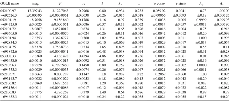
Because of the differences between WD and EBOP, we wish to compare only the geometric parameters of the solutions (see Paper I). Plotted in Fig. 2 are our values for the 81 binaries versus those of MiP05, for the sum of radii, inclination and eccentricity. The total radius and the eccentricity panels show quite small spread around the straight lines, which represent the locus of equal values of the two solutions. Only the inclination shows a large scatter and a slight bias. However, as noted above, our statistical analysis does not use the inclinations of the eclipsing binaries for the derivation of the characteristics of the short-period binaries. Therefore, the com-parison with the solutions of MiP05 supports our assessment that while individual EBAS solutions might be inferior to WD solutions, the statistical interpretation of the entire sample remains valid.

3 T R I M M I N G T H E S A M P L E

The very large sample of 1931 short-period binaries enables us to derive some statistical features of the population of short-period binaries in the LMC. However, the sample suffers from serious observational selection effects, which affected the discovery of the eclipsing binaries. To be able to correct for the selection effects, we need a well-defined homogeneous sample. We therefore trim

1_{http://wise-obs.tau.ac.il/∼omert/.}

the sample before deriving some parameter distributions in the next section.

The most important observational selection effect is associ-ated with the weak signal of the eclipse relative to the noise of the measurements. To apply a correction for this selection effect we need a distinct criterion that defines the systems that could have been detected by the OGLE LMC survey. Such a crite-rion is the detectability parameterD, which we define to be the number of points in the light curve, N, times the ratio of the

variance of the ideal but variable signal, to the variance of the residuals:

D=Nvar(mi)

var(ri)

, (3)

wheremi represent the values of the EBAS model at the times

of observation, andri are the residuals of the measurements

rel-ative to the model. One sees that systems with deep eclipses, which are more easily detected, have larger D, and even more so when many measurements are concentrated within phases of eclipses.

Fig. 3 shows the distribution of logDfor all 1931 solved systems. The histogram shows that there are only very few systems with logDbelow 2.6. We therefore set our detection limit, somewhat arbitrarily, at logD = 2.6, assuming that any binary below this limit could not have been detected. As pointed out by the referee, this limit translates intoD = 400, which implies a 1σ variation in a light curve having 400 points – a rather typical number. We consider the few systems below this limit as exceptions. In order to get a homogeneous sample, we ignore the binaries below this limit, and consider only the 1875 systems with logD>2.6.

Fig. 4 shows the total magnitude of the binaries left in the sam-ple as a function of their orbital periods. We are witnessing a lack of systems in the lower right-hand corner of the plot. This is due to the fact that the probability of having an eclipse is approxi-mately equal to the sum of fractional radii,rt. The two absolute radii determine the total luminosity of their system, while the bi-nary separation determines the orbital period. Therefore, for a given period, the probability of having an eclipse is smaller for faint sys-tems, with smaller stellar radii, than for brighter syssys-tems, with larger stars. In addition, the detectabilityDis smaller for fainter systems which have larger var(ri), making fainter systems less frequent in the

sample.

In order to obtain a sample that does not suffer from severe incom-pleteness, we chose, somewhat arbitrarily, to consider only systems in the range of total magnitude between 17 and 19 and with periods shorter than 10 d. The selected range, which included 1131 systems, is denoted in the figure.

For a distance modulus of μ0 = 18.50± 0.02 (Alves 2004), the trimmed sample range is between the absoluteI magnitude of −1.5 and 0.5, if interstellar absorption is neglected. For a metallicity

Z=0.008 (typical of the LMC), this range corresponds, for single stars at zero-age main sequence (ZAMS), to spectral type between B1 and B6 and mass range between 8.7 and 3.6 M(Schaerer et al. 1993). Obviously, if the two stars have close to equal luminosities, the primary could be as faint as 1.2 inI, which corresponds to a B8

spectral type.

Finally, we calculated for all binaries the averagedV−I colour

index. This was calculated by averaging allV measurements that

were observed in the phase between 0.15 and 0.35, and 0.65 and 0.85, that is out of eclipse. TheI magnitude of each system was

taken from the orbital solution. Fig. 5 presents for the 1931 binaries with reliable elements theI magnitude as a function of the averaged

Table 2. The 10 binaries: photometric elements.

OGLE name mag P rt k Js x e cosω e sinω Ap As

052100.97 17.397 43 3.122 7063 0.2968 0.80 0.934 0.233 0.059 02 0.0041 0.73 1.000 00 −692526.3 ±0.000 95 ±0.000 0061 ±0.0038 ±0.26 ±0.015 ±0.018 ±0.00066 ±0.0093 ±0.18 ±0.000 26 052101.19 18.7058 9.156 860 0.1788 1.16 0.97 0.339 −0.0038 0.005 0.9999 0.999 93 −694725.0 ±0.0025 ±0.000 051 ±0.0086 ±0.37 ±0.13 ±0.062 ±0.0014 ±0.057 ±0.0013 ±0.000 90 052101.72 18.0867 1.457 0012 0.674 1.31 0.65 0.696 0.0016 0.004 0.75 0.916 −693505.0 ±0.0015 ±0.000 0070 ±0.024 ±0.26 ±0.11 ±0.016 ±0.0042 ±0.012 ±0.20 ±0.099 052101.94 17.6753 1.362 6777 0.560 1.02 0.954 0.607 0.0003 0.011 1.000 0.998 −692834.5 ±0.0015 ±0.000 0025 ±0.015 ±0.10 ±0.069 ±0.019 ±0.0029 ±0.017 ±0.013 ±0.054 052104.75 18.5378 1.756 8736 0.534 1.65 0.895 −0.035 0.0002 −0.018 0.55 0.11 −691842.6 ±0.0023 ±0.000 0041 ±0.016 ±0.48 ±0.038 ±0.094 ±0.0032 ±0.028 ±0.31 ±0.28 053008.33 17.6360 4.136 428 0.4594 4.86 0.065 0.736 0.0006 −0.061 0.01 0.945 −693438.0 ±0.0010 ±0.000 015 ±0.0092 ±0.51 ±0.018 ±0.026 ±0.0052 ±0.028 ±0.16 ±0.099 052105.63 18.9528 6.799 2460 0.1450 0.80 0.757 0.275 0.0018 −0.002 1.0000 0.990 −694533.3 ±0.0029 ±0.000 0035 ±0.0074 ±0.26 ±0.076 ±0.047 ±0.0021 ±0.066 ±0.0011 ±0.038 052105.71 18.6663 8.000 289 0.1147 1.8 0.987 0.22 0.2069 −0.060 1.00 0.095 −693143.7 ±0.0022 ±0.000 029 ±0.0053 ±1.8 ±0.089 ±0.13 ±0.0012 ±0.042 ±0.20 ±0.040 052106.82 17.6869 1.699 1553 0.591 1.20 0.362 0.780 0.0015 0.031 0.988 0.820 −693136.4 ±0.0011 ±0.000 0086 ±0.017 ±0.12 ±0.094 ±0.018 ±0.0079 ±0.022 ±0.022 ±0.087 052106.83 17.5775 4.796 268 0.379 1.40 0.64 0.686 0.0029 −0.038 0.99 0.79 −694632.3 ±0.0011 ±0.000 024 ±0.010 ±0.24 ±0.22 ±0.035 ±0.0024 ±0.055 ±0.15 ±0.20

V −I colour. Obviously, most binaries are on the main sequence,

but some binaries are not. We excluded the binaries out of the plotted lines and were left with 938 binaries. This is the trimmed sample that the next section uses for the statistical analysis of the short-period binaries in the LMC.

4 S TAT I S T I C A L A N A LY S I S O F T H E T R I M M E D S A M P L E

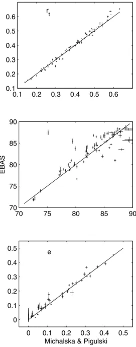
4.1 The radii and the surface brightness ratio distributions In order to study the statistical features of the short-period binaries in the LMC with mainly B-type main-sequence primaries, we plot-ted in Fig. 6 the distribution of four orbital elements derived for the trimmed eclipsing binary sample. This includes the surface bright-ness ratio of the two stars, the fractional primary and secondary radii, and the sum of the two radii.

The distributions are represented by histograms, which were de-rived by the Gaussian kernel method (e.g. Silverman 1986). Each binary is represented by a normal distribution centred on the derived value of its parameter, with a width equal to the estimated uncer-tainty of the parameter. Therefore, each of the histograms represents a sum of normal distributions, differing in mean and variance. The error bars in the histogram bins are just the square root of the value of each bin, assuming Poisson statistics.

Obviously, the observed distributions are highly convoluted by selection effects. For example, binary systems with longer periods must have an inclination closer to 90◦to be detected as an eclipsing binary. To correct for this effect, we calculated for each system the minimum inclination for which the eclipse could still be detected. This was done by calculating for each system the minimum incli-nationiminfor which the produced eclipse would still be above the detection threshold, given the physical parameters of the two stellar components and the binary elements. We assumed a light curve is detectable whenever logD>2.6, as above.

Assuming the systems are randomly oriented in space, the proba-bility of an inclination to fall betweeniminand 90◦isp=cosimin. To

account for systems with inclinations outside this range, we consid-ered each system as representing 1/p binaries, and drew the different

histograms accordingly.

Actually, the probability of detection might also be a function of the phase of the primary eclipse, especially if the data points are not equally distributed over the binary phase and the period is close to an integer number of days [see the discussion of Pont et al. (2005), and in particular their fig. 12]. We therefore averaged eachp over

100 different phases of the primary eclipse, and only then assigned each system with 1/p binaries.

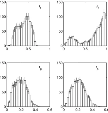
The histograms of the ‘weighted’ binaries are shown in Fig. 7. The error bars of each bin were calculated by taking the square root of the sum of squares of the 1/p values of that bin.

The histograms of the primary and secondary radii show a dra-matic rise between 0.05 and 0.1, and a moderate linear decrease be-tween 0.1 and 0.4. The distribution of the surface brightness ratios has a maximum at about unity and decreases monotonically down to about 0.5±0.1; then it reverses its trend, rising to a secondary, small maximum at about 0.2.

The histogram of the surface brightness ratios reflects the mass-ratio distribution of the whole population of short-period binaries with early-type primaries. This is especially true for main-sequence stars, where for a given primary star the surface brightness ratio of a binary is a monotonic function of its mass ratio. Therefore, the small local secondary maximum at 0.2 is of particular interest, because it might be an indication for a similar local maximum in the mass-ratio distribution.

However, the local maximum of the surface brightness ratio dis-tribution could have been caused by binaries that have gone through mass transfer. Such binaries should have relatively short periods. To follow the nature of the local small maximum, we plotted in Fig. 8 the corrected histograms only for the binaries with logP>0.5. The secondary peak at the distribution of the surface brightness ratios almost disappears, and the histogram decreases quite monotonically from the peak at unity. We, therefore, suggest that the initial mass-ratio distribution of the short-period binaries with B-type primaries rises monotonically up to a mass ratio of unity.

0.1 0.2 0.3 0.4 0.5 0.6 0.1 0.2 0.3 0.4 0.5 0.6 rt 70 75 80 85 90 70 75 80 85 90 i EBAS 0 0.1 0.2 0.3 0.4 0.5 0 0.1 0.2 0.3 0.4 0.5 _e

Michalska & Pigulski

Figure 2. Comparison with the work of MiP05: elements for 81 systems. Panels are for sum of radii, inclination and eccentricity.

4.2 The period distribution

To study the period distribution of the binaries in the LMC, we plotted in Fig. 9 period histograms of the trimmed sample, before and after the correction for the observational effects was applied. We emphasize that if the correction was applied properly, the lower panel represents the period distribution of all binaries in the LMC withI magnitude between 17 and 19, and with sum of radii smaller

than about 0.6, and not only the eclipsing binaries.

The corrected period histogram shows clearly a distribution that rises up to about logP=0.3, and then flattens off. However, before we conclude that this is the actual distribution of short-period bi-naries, we have to consider another possible selection effect, which is associated with the fact that the fractional length of an eclipse is shorter for long-period binaries than for short-period binaries. This effect turns the number of observations within an eclipse to

2 3 4 5 6 0 50 100 150 200 250 Log D

Figure 3. Distribution of the detectability parameter logDfor the 1931 binaries with acceptable solutions.

be smaller for long-period binaries than for short-period binaries. Therefore, for the same two stellar components and eclipse depth, the signal associated with the eclipse is smaller for binaries with long periods than for those with short periods. Consequently, the minimum secondary radius that can be detected might be a func-tion of the binary period. This might reduce the number of binaries discovered with long periods.

However, this selection effect can be substantial only for stars with small relative radii. Eclipsing binaries in our sample, with secondary radii larger than 0.03 and primary ones in the range 0.1–0.2, can be detected easily for periods of 10 d. We therefore suggest that the eclipse length effect should be quite small in our sample. To further check this point, we calculated how an assumed flat log distribution between 2 and 10 d would be affected by the eclipse length effect. To do that, we took all the 143 binaries in the sample with 0.3< logP<0.4 and checked their detectability if we change their period to be 10 d and their inclination to be 90◦. Only eight binaries lost

0 1 2 3 13 14 15 16 17 18 19 20 21 Log P Total Magnitude

Figure 4. Total I magnitude versus period for 1875 binaries with accepted solutions and high enough detectability. The straight lines present the limits of the trimmed sample. Periods are in d.

–0.5 0 0.5 1 1.5 2 14 15 16 17 18 19 20 21 V–I I

Figure 5. The I magnitude as a function of the averaged V − I colour.

Binaries excluded from the trimmed sample by the previous constraints are represented by dots. All 1131 binaries still in the trimmed sample are presented by small circles.

their detectability because of the eclipse length effect. This means that the implication of this effect is less than 6 per cent.

We therefore conclude that the period distribution of the short-period binaries is consistent witha flat log distribution between 2 and 10 d.

4.3 The frequency of the short-period binaries

As stated above, the corrections we apply allow us to study the distributions of all short-period binaries, up to 10 d, and not only the eclipsing binaries. We wish to take advantage of this feature of our analysis and estimate, within the limits of the sample, the total number of binaries in the LMC and their fractional frequency.

0 0.5 1 0 50 100 150 r t 0 0.5 1 0 50 100 150 J s 0 0.2 0.4 0.6 0 50 100 150 r p 0 0.2 0.4 0.6 0 50 100 150 r s

Figure 6. Histogram of the derived elements.

0 0.5 1 0 200 400 600 800 1000 r t 0 0.5 1 0 200 400 600 800 J s 0 0.2 0.4 0.6 0 200 400 600 800 1000 r_p 0 0.2 0.4 0.6 0 200 400 600 r_s

Figure 7. Histogram of the elements, corrected for the observational selec-tion effect.

The sum of weights of the 938 binaries in the trimmed sample is 4585. This means that we estimate there are 4585 short-period binaries in the LMC that fulfil the constraints we have on the trimmed sample. To get the total number of binaries with periods shorter than 10 d, we have to add the high-alarm binaries and the ones with large radii; since the added systems are close binaries, their detection probability reaches almost 1 so we do not correct for it in their case. When we add those, we end up with 5004 binaries.

We therefore suggest that the number of binaries in the LMC, with period shorter than 10 d, withI between 17 and 19, and for

0 0.5 1 0 200 400 600 r t 0 0.5 1 0 100 200 300 400 J s 0 0.2 0.4 0.6 0 200 400 600 r_p 0 0.2 0.4 0.6 0 100 200 300 400 r_s

0 0.2 0.4 0.6 0.8 1 0 20 40 60 Log P (days) 0 0.2 0.4 0.6 0.8 1 0 100 200 300 400 Log P (days)

Figure 9. The period distribution of the binaries in the LMC. The top panel shows the period histogram of the trimmed sample, while the lower one shows the corrected histogram

which theV − I colour of the system indicates a main-sequence

primary, is about 5000.

Our estimate is valid as far as Wyrzykowski et al. (2003) detected all eclipsing binaries and classified them as such, rather than as other types of variables (e.g. small amplitude Cepheids). We do correct for the detection probability, including for the effect of phase of minima, but still assumed that each binary has been correctly identified. One could imagine that 10 to 30 per cent of the potentially detectable binaries were missed for some reason, but hardly much more. We, therefore, arbitrarily assign an error of 30 per cent to the number of binaries in the sample.

We have shown that our sample consists mainly of B-type main-sequence binaries. In order to estimate the fractional frequency of B-type main-sequence stars which reside in binaries that could have been detected by OGLE, we have to estimate how many main-sequencesingle stars were found by OGLE in the same range of

magnitudes and colours. To do that, we applied exactly the same procedure we performed above to the whole OGLE data set of LMC stars in the 21 OGLE fields and found 332 297 main-sequence stars in the I range of 17–19. However, the luminosity of a binary is

brighter than the luminosity of its primary by a magnitude that depends on the light ratio of the two stars of the system. Therefore, to consider a population of single stars which is about equal to the population of the primaries of our binary sample we considered instead the range between 17.5 and 19.5 I magnitude, and found

705 535 stars. Taking into account about 1 per cent overlap between the OGLE fields, we adopt 700 000 as a representative number of

17 17.5 18 18.5 19 0 0.1 0.2 0.3 0.4 0.5 0.6 0.7 0.8 0.9 1 mag Survey Binaries

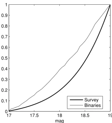
Figure 10. The magnitude cumulative distribution functions of the LMC binaries and the entire LMC survey. To show comparable populations, we plot the distribution of binaries between 17 and 19I magnitude and of stars

between 17.5 and 19.5.

single stars in the LMC similar to the population of our binary sample. We arbitrarily assign an error of 50 per cent to this figure.

We therefore conclude that (0.7 ± 0.4) per cent of the main-sequence B-type stars in the LMC are found in binaries with periods shorter than 10 d.

A question that naturally arises is whether the binary frequency depends on the mass of the components. While the answer to this question is outside the scope of this study, our results allow us to examine the variation of the binary frequency in a small magnitude range. In Fig. 10, we plot the magnitude cumulative distribution functions of both the binaries and of the entire survey. To display comparable populations, we plot the distribution of binaries between 17 and 19I magnitude and of stars between 17.5 and 19.5. While

the stellar magnitude distribution rises exponentially, the binary dis-tribution is almost linear. Hence, the frequency of binaries is higher for brighter stars. In fact, the frequency of binaries in the magnitude range 17–18 is 1.5 per cent, while the frequency between 18 and 19 is 0.5 per cent – a factor of 3 smaller. It is also difficult to see how the very strong variation of the rate of binaries with magnitude range could be credited to detection incompleteness only, so we suggest it is real.

4.4 The eccentricity distribution

Another feature of the whole sample that we wish to touch upon is the dependence of the binary eccentricity on the total radius. North & Zahn (2004) ignored the Algol-type eclipsing binaries of Wyrzykowski et al. (2003), and considered only eclipsing binaries that did not show considerable variation out of the eclipse. We, on the other hand, consider here all binaries with sum of radii smaller than 0.6, and therefore, naturally, have more systems with larger fractional averaged radii.

0.2

0.4

0.6

0.8

–0.4

–0.2

0

0.2

0.4

0.6

r

e cos

ω

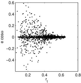
Figure 11. e cosωversus the total radius.

Following North & Zahn (2003), Fig. 11 shows the eccentricity, multiplied by cosω, as a function of the sum of radii. There are two minor differences between our figure and that of North & Zahn (2003). First, we present the sum of radii, while North & Zahn (2003) presented the radius, which is probably close to the average radius, as they used a value of unity for the radius ratio, and did not allow the ratio to change. Secondly, we use the value of cosω, while North & Zahn (2003) plotted the absolute value of this parameter. Despite these minor differences, the result obtained here is quite similar to the work of North & Zahn (2004), who found the value of the limitingaveraged radius to be 0.25.

5 D I S C U S S I O N 5.1 The period distribution

Our analysis suggests that the binaries with B-type primaries in the LMC have flat log-period distribution between 2 and 10 d. This distribution, which was obtained after correcting for observational selection effects, is very different from the distributions of the whole samples of the SMC and the LMC eclipsing binaries (Udalski et al. 1998; Wyrzykowski et al. 2003). Evidently, correcting for the se-lection effects reveals a substantially different period distribution.

The period distribution derived here is probably not consistent with the period distribution of Duquennoy & Mayor (1991), who adopted a Gaussian with logP=4.8 andσ=2.3,P being measured

in days. Their distribution would provide within a logP interval

almost twice as many systems at logP=1.0 than at logP=0.3 (more precisely, the factor would be 1.7), while the new derived distribution is probably flat.

It is interesting to note that Heacox (1998) reanalysed the data of Duquennoy & Mayor (1991) and claimed thatf (a), the distribution

of the G-dwarf orbital semimajor axis,a, is f (a)∝a−1_{da, which} implies a flat log orbital separation distribution. This is equivalent to the present probable result, although the latter refers to LMC binaries with B-type primaries, and is limited only to a very small range of orbital separation. On the other hand, Halbwachs et al. (2003, hereafter HaMUA03) analysed the spectroscopic binaries

found within the G and K stars in the solar neighbourhood and the ones found in the Pleiades and Praesepe, and found that the log-period distribution is ‘clearly rising until about 10 days’.

However, HaMUA03’s sample included only a few systems with periods longer than 2 d and shorter than 10 d. Actually, there were seven such systems in the ‘extended sample’ of nearby stars and five additional binaries in the Pleiades and Praesepe. In fact, if we divide these 12 binaries into two bins with equal log width, then we find six in the short-period bin and six in the long-period one. It is true that the correction factor of the spectroscopic binaries of these two bins is somewhat different, and therefore the distribution of this sample might still be consistent with the conclusion of HaMUA03. However, the small number of binaries with periods shorter than 10 d in the G and K binaries is also consistent with flat log distribution below 10 d. We verified that by building the cumulative distribution of the logP values of the 12 G and K binaries, and comparing it with

the theoretical flat log distribution. The one-sided Kolmogorov– Smirnov test gives a probability of 0.7 that the observed distribution is consistent with the flat log distribution.

The flat log-period distribution implies a flat log orbital-separation distribution for a given total binary mass. Such a distribu-tion indicates that there is no preferred length-scale for the formadistribu-tion of short-period binaries (Heacox 1998), at least in the range between 0.05 and 0.16 au, for a total binary mass of 5 M. Alternatively, the results indicate that the specific angular momentum distribution is flat on a log scale at the 1019_cm2_s−1_range.

A note of caution is in order here, as the present analysis refers toall eclipsing binaries in a given absolute magnitude range. Even

if the overwhelming majority of the binaries lie on or close to the main sequence, a small unknown number of them may have gone through a mass-exchange phase, which would have affected both the orbital period and the stellar radii. This is very important for the interpretation of the new result, since the most interesting quantity is probably theprimordial period distribution, which was not

af-fected by the subsequent binary evolution. In fact, Harries, Hilditch & Howarth (2003) and Hilditch, Howarth & Harries (2005, here-after HiHoHa05) studied in details 50 eclipsing binaries in the SMC and found more than half of them to be in a semi-detached post-mass-transfer state. However, the binaries studied in the SMC, with limiting brightness ofB<16, are brighter than the systems in the trimmed sample, and are composed mainly of O to B1-type pri-maries, while most of the primaries in the present sample are cooler B-type stars. Apparently, the fractional radii of the stars studied by HiHoHa05 is substantially larger than the typical fractional radii of the present sample. We therefore suggest that while a large fraction of the HiHoHa05 sample has gone through mass exchange, most of the binaries studied here are still on the main sequence.

We therefore suggest that the short-period B-type binaries in the LMC might have had a primordial flat log-period distribution be-tween 2 and 10 d, and a similar featurecould have been found in

binaries with G-type primaries in the solar neighbourhood. Although this probable result refers to a very narrow period range, a binary for-mation model should account for this scale-free distribution, which might be common in short-period binaries.

5.2 The binary fraction

It would be interesting to compare the frequency of B-star bina-ries found here for the LMC with a similar frequency study of B stars in our Galaxy. However, such a large systematic study of eclipsing binaries is not available. Instead, a few radial-velocity and photometric searches for binaries in relatively small Galactic

samples were performed. In what follows, we compare the frequency derived here with results of radial-velocity searches for binaries, in samples of Galactic B stars as well as within the nearby K and G stars. In addition, we discuss the binary frequency found by the

Hubble Space Telescope (HST) photometric monitoring of 47 Tuc.

5.2.1 Radial-velocity searches for binaries

Wolff (1978) studied the frequency of binaries in sharp-lined B7–B9 stars. Her table 1 presents 73 such stars withV sin i<100 km s−1_, among which 17 are members of binary systems with Porb < 10 d. This represents a percentage of 23 per cent, much larger than the frequency we find in the LMC. On the one hand, the frequency of Wolff (1978) may be considered a lower limit, since her sample was biased towards sharp-lined stars, because her purpose was to deter-mine what fraction of the intrinsically slowly rotating B stars are members of close binary systems. This introduced a bias towards lowV sin i values and therefore small orbital inclinations, hence

lower detection probabilities, assuming the spin and orbital axes are aligned. On the other hand, the sample is magnitude limited, but the correction for the Branch bias (Branch 1976) was not applied. The most extreme correction factor for the bias towards the more luminous binary systems, which holds for systems with two identi-cal components, is f=0.35. Applying this factor to the rate of late B-type binaries with Porb<10 d leaves a minimum frequency of 8±2 per cent. This remains one order of magnitude larger than our frequency in the LMC.

Similar and even higher values of binary frequency were derived for B stars in Galactic clusters and associations. Morrell & Levato (1991) have determined the rate of binaries among B stars (a few O and A-type stars are also included in the sample) in the Orion OB1 association, and obtained an overall frequency of binaries with

Porb<10 d of 26±6 per cent. There is a slight trend towards a higher rate of binaries among the early B stars than among the late ones. For B4 and earlier stars, they found 60 per cent binaries, while only∼27 per cent of the B5 and later stars were found to be radial velocity variables, which is reminiscent of what we find in the LMC. However, this is hardly significant as the latter frequency is based only on three variables.

Garcia & Mermilliod (2001) found a rate of binaries as high as 82 per cent among stars hotter than B1.5 in the very young open cluster NGC 6231, though in a sample of 34 stars only. Most orbits have periods shorter than 10 d. Raboud (1996) estimated a rate of binaries of at least 52 per cent for 36 B1–B9 stars in the same cluster, but his data did not allow him to determine the orbital periods.

These studies show that binaries hosting B-type stars tend to be more frequent in young Galactic clusters than in the field. However, even though our LMC binaries are the representatives of the LMC field rather than of LMC clusters, the frequency we derived appears much lower than that of the binaries in the Galactic field.

One survey of a complete, volume-limited sample of binaries in the solar neighbourhood is that of HaMUA03, who carefully studied a complete sample of K- and G-type stars, and not B stars. Out of a bias-free sample of 405 in the solar neighbourhood, they found 52 binaries, 11 of them with periods shorter than 10 d. This results in a fractional frequency of (2.7± 0.8) per cent binaries, if one takes just the Poisson distribution to estimate the error. We therefore suggest that the fractional frequency of K- and G-type stars in the solar neighbourhood found in binaries with periods shorter than 10 d is higher by a factor of about 3.9±1.9 than the corresponding frequency of B-type stars in the LMC. The error estimate of the factor

between the two fractional frequencies was derived by assuming normal distribution, and is only a coarse estimate, because of the small number statistics of the K- and G-type binaries. In fact, the difference between the two fractional frequencies is at about the 2σ level.

5.2.2 HST photometric monitoring of 47 Tuc

A few photometric studies were devoted to the search of eclips-ing binaries in Galactic globular clusters (e.g. Yan & Reid 1996; Kaluzny et al. 1997). One of the recent photometric studies is the

HST 8.3-d observations of 47 Tuc (Albrow et al. 2001), which

mon-itored 46 422 stars in the central part of the cluster and discovered 5 eclipsing binaries with periods longer than about 4 d. Assuming a flat log-period distribution of binaries, Albrow et al. (2001) con-cluded that the primordial binary frequency up to 50 yr was (13± 6) per cent. This estimate translates into (2±1) per cent for periods between 2 and 10 d. This value, derived for late-type stars, is much smaller than the frequency derived by the radial-velocity surveys of B stars, and is close to the (0.7±0.4) per cent frequency we derived for the LMC.

5.2.3 Comparison between the two approaches

We conclude that the frequency of binaries we find in the LMC is substantially smaller than the frequency found by Galactic radial-velocity surveys. The detected frequency of B-type binaries is larger by a factor of 10 or more than the frequency we find, while the binary frequency of K- and G-type stars is probably larger by a factor of 4. On the other hand, the binary frequency found by photometric searches in 47 Tuc is only slightly higher and still consistent with the frequency we deduced for the LMC. It seems that the frequency derived from photometric searches is consistently smaller than the one found by radial-velocity observations.

We are not aware of any observational effect that could cause such a large difference between the radial velocity and the photo-metric studies. The sensitivity of the two approaches depends on the ability to discover binaries with secondaries of small radii, in the photometry case, and small masses, in the case of the radial-velocity searches. In order to account for the large differences between the photometric and the spectroscopic searches, we have to assume that the photometric searches detect only 10 per cent of the binaries and missed all the others, that could have been discovered by radial-velocity techniques. Although Wolff (1978) suggested that many short-period binaries in her radial-velocity sample have low-mass secondaries, this effect cannot explain a factor of 10 in the detected frequency. The discussion of the distribution of radii of our sample also indicates that if such an effect is present in the LMC binaries it must be small. After all, the radial-velocity searches are not sen-sitive to small-mass secondaries, and they too suffer from selection effects which depends on their precision. Therefore, the large dif-ference in the binary frequencies is probably real and remains a mystery. Obviously, it would be extremely useful and interesting to have studies of eclipsing binaries similar to the present one in our Galaxy, as well as in other nearby galaxies.

5.3 The stellar radii and the surface brightness ratios

The distributions of the two fractional radii depend strongly on the derivation of the ratio of radii, which is not well determined from the light curves. Still, a statistical analysis of the distributions is meaningful, given the high correlation between the true and derived

k values, as shown in the simulations in Paper I. The distributions of

the radii show sharp peaks at the same value of 0.1, as can be seen in Fig. 7, and in Fig. 8 in particular. This suggests, but admittedly does not prove, that our sample is mostly composed of stars with similar radii. The distribution ofJs tends to reinforce this interpretation, since it suggests a mass ratio – hence a ratio of radii – close to one. For the primary, the rise between 0.05 and 0.1 is due essentially to the limit imposed on the orbital period and to the minimum ra-dius of a star on the ZAMS. On the other hand, the sharp rise of the secondary radius distribution up to a radius of about 0.1 is probably real. This feature of the secondary radius distribution could have been the result of a selection effect – too small a secondary results in an eclipse too shallow to be detected by the OGLE photome-try. We suggest that this is not the case. The detectability limit of the sample is such that any binary with eclipse deeper than about 0.1 mag, corresponding to 10 per cent drop in the system brightness, is included in the sample. Such a drop can be caused by a secondary with a radius which is about 0.3 of the primary radius, for inclination of 90◦andJs<1. If the primary radius peaks at∼0.1, the sample is then complete for secondary radius down to about 0.03.

The peaks at about 0.1 in Fig. 8 indicate that a substantial fraction of the primary and the secondary stars in the sample have radius of 2.5–3 R, assuming a typical period of 7 d in Fig. 8 and a typical mass of 5 M. The sharpness of the peaks is probably caused by the magnitude limits of the trimmed sample.

5.4 The eccentricity distribution

Fig. 11, with the eccentricity as a function of the sum of the two radii, displays upper and lower envelopes that can be approximated with two straight lines, with a slope of about 1.7 in absolute value. Al-though both the shape and slope of these envelopes may be plagued by selection biases, it is interesting to remark that the populated area corresponds to the condition

rt=rp+rs0.59 (0.85− |e cosω|). (4) This roughly generalizes the conditionraverage0.25 to the case of eccentric systems, which cannot keep an eccentricity larger than some limiting value. This limiting value of the eccentricity depends on the stellar radii, whose sum cannot be larger than a given critical fraction of the distanceat periastron. Because of the cosωfactor, it is reasonable to assume that the real relation is rather

rp+rs0.5 (1−e).

Systems with eccentricities larger than that will undergo partial tidal circularization until they satisfy this inequality; after that, tidal ef-fects become almost inefficient. The boundary is clear-cut even though the systems do not share the same age, due to the very steep dependence of circularization time on relative radius:tcirc∝ (R/a)−21/2(Zahn 1975, 1977).

Note also that there are quite a few binaries with small radii for which the parametere cosωis very close to zero. It is difficult to assume that all these systems have cosω=0. Probably those systems have circular orbits. It would be interesting to find out whether these systems were circularized during their main-sequence phase, despite their small radii, or maybe their very small eccentricity is primordial.

6 S U M M A RY

The OGLE data set has allowed us to analyse for the first time the statistical characteristics of short-period binaries with B-type

pri-maries of an entire galaxy. We analysed the 2580 eclipsing LMC light curves found by Wyrzykowski et al. (2003) and obtained or-bital elements for 1931 systems. We further derived some statistical features of a trimmed sample of 938 binaries with periods shorter than 10 d, main-sequence primaries, andI magnitude between 17

and 19. After correcting for the inclination effect, we find that the log-period distribution of the short-period binaries is probably flat between 2 and 10 d. Finally, we suggest that (0.7±0.4) per cent of the main-sequence B-type stars in the LMC are found in binaries with periods shorter than 10 d. This is substantially smaller than the fraction found in the nearby K- and G-type stars and much smaller than that of nearby B stars. We are preparing another paper on the distribution of stars in the SMC, to find out the metallicity effect of the frequency of binaries.

This work is a further step in the study of the extragalactic binaries. Most previous studies concentrated on individual systems [see a review by Ribas (2004), and references therein]. The photometry of a whole galaxy, the LMC in our case, can provide photometry of thousands of eclipsing binaries, together with distance modulus which is common to all binaries in the same galaxy. The known distances to the galaxies in the Local Group can provide us with absolute magnitude for a large set of early-type eclipsing binaries that is not available for Galactic binaries. Therefore, the statistical analysis of the extragalactic binaries presents great potential to our understanding of the formation of early-type binaries and stellar models.

AC K N OW L E D G M E N T S

We are grateful to the OGLE team, and to L. Wyrzykowski in partic-ular, for the excellent photometric data set and the eclipsing binary analysis that was available to us. We thank J. Devor, G. Torres and I. Ribas for very useful comments. The remarks and suggestions of the referee, T. Zwitter, helped us to substantially improve the algo-rithm and this paper. This work was supported by the Israeli Science Foundation through grant no. 03/233.

R E F E R E N C E S

Albrow M. D., Gilliland R. L., Brown T. M., Edmonds P. D., Guhathakurta P., Sarajedini A., 2001, ApJ, 559, 1060

Alcock C., Allsman R. A., Alves D., Axelrod T. S., Becker A. C., 1997, AJ, 114, 326

Alves D. R., 2004, New Astron. Rev., 48, 659 Branch D., 1976, ApJ, 210, 392

Devor J., 2005, ApJ, 628, 411

Duquennoy A., Mayor M., 1991, A&A, 248, 485 Eggleton P. P., 1983, ApJ, 268, 368

Garcia B., Mermilliod J.-C., 2001, A&A, 368, 122

Gonz´alez J. F., Ostrov P., Morrell N., Minniti D., 2005, ApJ, 624, 946 Halbwachs J. L., Mayor M., Udry S., Arenou F., 2003, A&A, 397, 159

(HaMUA03)

Harries T., Hilditch R., Howarth I., 2003, MNRAS, 339, 157 Heacox W. D., 1998, AJ, 115, 325

Hilditch R., Howarth I., Harries T., 2005, MNRAS, 357, 304 (HiHoHa05) Kaluzny J., Krzeminski W., Mazur B., Wysocka A., Stepien K., 1997, Acta

Astron., 47, 249

Michalska G., Pigulski A., 2005, A&A, 434, 89 (MiP05) Morrell N., Levato H., 1991, ApJS, 75, 965

North P., Zahn J.-P., 2003, A&A, 405, 677

North P., Zahn J.-P., 2004, New Astron. Rev., 48, 741

Pont F., Bouchy F., Melo C., Santos N. C., Mayor M., Queloz D., Udry S., 2005, A&A, 438, 1123

Raboud D., 1996, A&A, 315, 384 Ribas I., 2004, New Astron. Rev., 48, 731

Schaerer D., Meynet G., Maeder A., Schaller G., 1993, A&AS, 98, 523 Silverman B. W., 1986, Density Estimation for Statistics and Data Analysis.

Chapman & Hall, London

Tamuz O., Mazeh T., North P., 2006, MNRAS, in press (Paper I, this issue), doi:10.1111/j.1365-2966.2006.10049.x

Udalski A., Soszynski I., Szymanski M., Kubiak M., Pietrzynski G., Wozniak P., Zebrun K., 1998, Acta Astron., 48, 563

Udalski A., Szymanski M., Kubiak M., Pietrzynski G., Soszynski I., Wozniak P., Zebrun K., 2000, Acta Astron., 50, 307

Wolff S. C., 1978, ApJ, 222, 556

Wyithe J. S. B., Wilson R. E., 2001, ApJ, 559, 260 Wyrzykowski L. et al., 2003, Acta Astron., 53, 1 Yan L., Reid I. N., 1996, MNRAS, 279, 751 Zahn J.-P., 1975, A&A, 41, 329

Zahn J.-P., 1977, A&A, 57, 383

Zahn J.-P., Bouchet L., 1989, A&A, 223, 112 Zebrun K. et al., 2001, Acta Astron., 51, 317 S U P P L E M E N TA RY M AT E R I A L

The following supplementary material is available for this article online:

Table 3. Observations and goodness-of-fit for all binaries found. Table 4. Photometric elements for all binaries found.

This material is available as part of the online article from http://www.blackwell-synergy.com