Munich Personal RePEc Archive
Equilibrium Vengeance
Friedman, Daniel and Singh, Nirvikar
University of California, Santa Cruz
June 2007
Equilibrium Vengeance
Daniel Friedman and Nirvikar Singh
Economics Department
University of California, Santa Cruz
June 2007
Abstract
The efficiency-enhancing role of the vengeance motive is illustrated in a simple social dilemma
game in extensive form. Incorporating behavioral noise and observational noise in random
in-teractions in large groups leads to seven continuous families of (short run) Perfect Bayesian
equilibria (PBE) that involve both vengeful and non-vengeful types. A new long run
evolu-tionary equilibrium concept, Evoluevolu-tionary Perfect Bayesian Equilibrium (EPBE), shrinks the
equilibrium set to two points. In one EPBE, only the non-vengeful type survives and there are
no mutual gains. In the other EPBE, both types survive and reap mutual gains.
Keywords: reciprocity, vengeance, evolutionary perfect Bayesian equilibrium, social dilemmas.
JEL codes: C73, Z13
∗We are grateful to Matt McGinty for patient research assistance, and we benefited from helpful comments of seminar participants at UC Berkeley, UC Riverside, UC Santa Cruz, USC and Yale, and readers of earlier versions of
the paper. In particular, we thank Joshua Aizenman, Steve Goldman, Steffen Huck, Bentley MacLeod, Steve Morris,
1
Introduction
Craving vengeance is a powerful human motive: when some culprit harms you or your loved ones,
you may choose to incur a substantial personal cost to harm him in return. There can be major
economic and social consequences, positive and negative. Economic theory has not yet fully come
to grips with such motives. In this paper we model vengeance as an emotional state dependent
utility component and investigate its efficiency impact and its viability.
A taste for vengeance, the desire to “get even,” is so much a part of daily life (and the evening
news) that it is easy to miss the evolutionary puzzle. We shall argue that indulging one’s taste
for vengeance in general reduces one’s material payoff or fitness. Absent countervailing forces, the
meek (less vengeful people) should have inherited the earth long ago, because they had higher
fitness. Why then does vengeance persist?
To investigate the question, we introduce a new equilibrium concept,1 evolutionary perfect
Bayesian equilibrium (EPBE), that seems germane in a wide variety of applications. EPBE extends
the equal profit condition of competitive markets into games of incomplete information with possible
entry, exit and/or switching among multiple player types. Our paper uses EPBE to show how
vengeance can persist despite its apparent fitness handicap.
Vengeance is closely tied to several vexing issues, methodological and substantive. Therefore
we begin in Section 2 with a preliminary discussion on the nature of social dilemmas, the meaning
of positive and negative reciprocity, why both are important to economists, and various
model-ing approaches. Our contribution to this literature is to demonstrate the viability of a taste for
vengeance even when people interact in unstructured large groups, and the degree of vengefulness
is continuously variable and imperfectly observed.
Section 3 presents the basic social dilemma as a simple extensive form game, and shows how
vengeful preferences can dramatically improve equilibrium efficiency. It spotlights the
evolution-ary problem when an individual’s vengefulness cannot be perfectly known in advance and when
behavioral errors are possible. Finally, it argues for a simplification of the analysis: of all possible
distributions in continuous type space, it suffices to look only at those supported on just two points.
Section 4 derives seven continuous families of perfect Bayesian equilibria (PBE): two pooling
equilibria, one separating equilibrium, two mixed equilibria and two hybrids. The PBE are
short-run in that the nature and proportions of all player types are fixed. Section 5 examines the long-short-run
in which the nature and proportions of types can evolve. We define EPBE and show that in our
game it refines the equilibrium set from seven families down to two points: a unique EPBE that
1
As noted in concluding discussion and in the Appendix, Abreu and Sethi (2003) independently use essentially
supports social gains (characterized in Proposition 2, our central result), and a trivial, inefficient
EPBE (also in Proposition 2). A concluding section discusses generalizations and emergent issues.
The Appendix collects the mathematical details.
2
Preliminaries
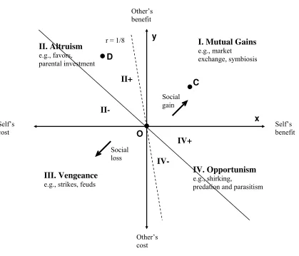
An action has a social dimension when it affects non-actors as well as the actor. Figure 1 lays out
the possibilities in terms of the net material benefit (x >0) or cost (x < 0) to the actor, denoted
“Self,” and the net material benefit (y > 0) or cost (y < 0) to counterparties, denoted “Other”.
Economists think most often about the mutual gains quadrant I, where actions simultaneously
benefit Self and Other. Such symbiotic actions increase social efficiency.
Quadrant IV is the well-studied opportunistic region, where Self benefits at Other’s expense;
the biological terms are parasitism and predation. The flip side is the altruism quadrant II, where
Self bears a personal cost in order to benefit Other. Quadrant III is especially interesting to us.
Cipolla (1976) refers to actions producing such outcomes as stupidity, but vengeance often will be
a better explanation.
Social dilemmas arise from the fact that evolution directly supports behavior that benefits Self,
i.e., outcomesx >0 in quadrants IV (or I) but not x <0 in II (or III), while in contrast, efficiency
requires outcomes above the diagonal [x+y = 0].2 Social creatures (such as humans) thrive on
devices that support outcomes in the half-quadrant II+ and discourage outcomes in IV-. Such
devices somehow internalize Other’s costs and benefits.
———–fig 1 about here———–
2.1 Efficiency-enhancing devices
Biologists emphasize the role of genetic relatedness.3 If Other is related to Self to degreer >0, then
a positive fraction of Other’s payoffs are internalized via “inclusive fitness” (Hamilton, 1964) and
evolution favors outcomes above the line [x+ry= 0]. For example, the unusual genetics of insect
order hymenoptera producer up to 34 between sisters; most social insects (including ants and bees)
belong to this order and the workers are indeed sisters. For humans and most other species, r is
2
More precisely, Self’s iso-fitness curves are the vertical linesx=C while iso-efficiency curves are diagonal lines
x+y=C. The status quo point (0, 0) ensures thatC≥0 is feasible.
3
Bergstrom (2002) and Robson (2002) provide excellent summaries of recent biological insights into economic
behavior. Henrich (2004) and subsequent articles in the special issue of JEBO dissect the biological and cultural
basis of human cooperation. Henrich also notes the limited scope of standard inclusive fitness and folk theorem
only 12 for full siblings and for parent and child, is 18 for first cousins, and goes to zero exponentially
for more distant relations. On averager is small in human interactions, as in the steep dashed line
in Figure 1, since we typically have only a few children but work and live in groups with dozens of
individuals. Clearly other devices are needed to support human social behavior.
Economists emphasize devices based on repeated interaction, as in the “folk theorem” (e.g.,
Fudenberg and Maskin, 1986). Suppose that Other returns the benefit (“positive reciprocity”)
with probability and delay together summarized in discount factorδ∈[0, 1). Then that fraction of
other’s payoffs are internalized (Trivers, 1971) and evolution favors behavior producing outcomes
above the line [x+δy = 0]. This internalization can support a large portion of socially efficient
behavior when δ is close to 1, i.e., when interactions between two individuals are symmetric,
predictable, frequent and ongoing.4 But humans specialize in exploiting once-off opportunities
with a variety of different partners, in which case δ is small, as in the same steep dashed line.
Other devices are needed to explain cooperation in such situations.
Here we will emphasize devices based on other-regarding preferences. For example, suppose
Self gets a utility increment of ry from his or her action,5 in addition to the material benefit x.
Hence Self partially internalizes the material externality, and undertakes behavior that is above the
line [x+ry= 0]. Friendly preferences, r ∈ [0, 1], thus can explain the same range of behavior as
genetic relatedness and repeated interaction. However, by itself the friendly preference device is
evolutionarily unstable: those with lower positiverwill tend to make more personally advantageous
choices, gain higher material payoff (or fitness), and displace the more friendly types. Friendly
preferences therefore require the support of other devices.
Vengeful preferences rescue friendly preferences. Self’s material incentive to reducerdisappears
when others base their values ofron Self’s previous behavior and employr <0 if Self is insufficiently
friendly. Such visits to quadrant III will reduce the fitness of less friendly behavior and thus boost
friendly behavior.6 But visits to quadrant III are also costly to the avenger, so less vengeful
preferences seem fitter. What then supports vengeful preferences: who guards the guardians? This
question motivates the present paper.
4
See Sethi and Somanathan (2003) for an extended discussion and survey of this device from the perspective of
evolutionary game theory. Our own approach may be seen as complementary to the analysis of repeated interactions,
covering different circumstances.
5
Rilling et al (2002), was among the first studies to present physiological evidence for such increments, based on
fMRI brain scans of subjects playing prisoner’s dilemma.
6
This idea is developed in the altruistic punishments literature (e.g., Fehr and Gachter, 2002; Boyd et. al, 2003).
2.2 Modeling other regarding preferences
Two main modeling approaches can be distinguished in the recent literature. The distributional
preferences approach7 begins with a standard selfish utility function and adds additional terms
capturing Self’s response to how own payoff compares to Other’s payoffs. The psychological games
approach captures reciprocity by postulating that my preferences regarding your payoff depend on
my beliefs about your intentions.8
We favor an alternative approach, inspired by the pioneering work of Hirshleifer (1987) and
Frank (1988). Model reciprocal preferences as state dependent: my attitude towards your payoffs
depends on my emotional state, e.g., friendly or vengeful, and your behavior systematically alters
my emotional state. Cox et al. (2007) show that a 3 or 4 parameter model incorporating this
approach accounts well for existing laboratory data.9 Fortunately, a very simple rule suffices for
present purposes: you become vengeful towards those who betray your trust, and otherwise have
standard selfish preferences.
To be convincing, a model of other regarding preferences must account for the empirical data
and also should pass the following theoretical test: people with the hypothesized preferences receive
at least as much material payoff (or evolutionary fitness) as people with alternative preferences.
This test is referred to as indirect evolution (G¨uth and Yaari, 1992; precursors include Becker, 1976,
and Rubin and Paul, 1979) because evolution operates on preference parameters that determine
behavior rather than directly on behavior.
The evolutionary test is prominent in a number of recent papers,10, several of which bear directly
on present concerns. Huck and Oechssler (1999) show that vengeance can survive in small groups,
where a vengeful person can impair others’ fitness more than his own. Herold (2003) shows that
positive as well as negative reciprocity (vengeance) can survive in a ”haystack” model, in which
people interact in small groups that are occasionally remixed. Our concern, however, is with large
unstructured populations.
In his introduction to the literature, Samuelson (2001) offers two challenges: can the
hypothe-7
This approach is exemplified in the Fehr and Schmidt (1999) inequality aversion model, the Bolton and Ockenfels
(2000) mean preferring model, and the Charness and Rabin (2002) social maximin model.
8
Building on the Geanakoplos, Pearce and Stacchetti (1989) model, Rabin (1993) constructs reciprocity equilibria
for two player normal form games, and Dufwenberg and Kirchsteiger (2004) and Falk and Fischbacher (2006) adapt
the idea to extensive form games. Levine (1998) improves tractability by replacing beliefs about others’ intentions
by estimates of others’ type.
9
A psychological theory of how emotional states change (e.g., van Winden, 2001) rounds out this approach; see
also Gintis (2002) and Sobel (2005).
10
For example, Dekel, Ely and Yilankaya (1998), Ely and Yilankaya (2001), Kockesen, Ok and Sethi (2000),
sized preferences emerge when there is a full range of alternatives, not just a handful, and can they
emerge when they are not perfectly observable? The first challenge is especially acute here because
many previous models of negative reciprocity are susceptible to unraveling: slightly lesser degrees
of vengefulness have higher fitness. Heifetz et al. (2007) is an important exception. They show
in great generality that, given observability, some distortion of selfish preferences (what they call
dispositions) generically survives evolutionary pressure. They also consider imperfect observability,
but only in a special case that assumes that Bayesian Nash Equilibria are locally unique and that
perceptual errors are uniformly bounded, neither of which holds in the model we present below.
Bohnet et. al (2001, Appendix A) sketch a model with imperfect type observability, but again it
covers only a special case that lies outside our present concerns. Like us, G¨uth et. al (2000)
exam-ine observability in a trust game, but it takes a quite different form. They analyze the fraction of
players with ”moral” dispositions and the fraction adopting a perfect but costly observation
tech-nology. As Samuelson notes, evolution favors those who can appear more committed (i.e., vengeful
in our context) than they really are, so perfect observability seems unrealistic.
To summarize, within existing literature on other regarding preferences, our paper is
distin-guished by its focus on: (a) vengeance, a contingent preference for costly punishment. The
ma-jority of papers focus on noncontingent preferences (or dispositions), or on positive reciprocity.
(b) Evolution in large unstructured populations, a more challenging and general environment. (c)
Imperfect observability, responding to Samuelson’s second challenge. Players never know for sure
how vengeful their partners might be. (d) A continuum of types. In response to Samuelson’s first
challenge, we want to show that a greater or lesser degree of vengefulness will not lead to higher
material payoffs.
3
The Underlying Game
The first step in analyzing social preferences is to model explicitly the underlying social dilemma.
We use a simple extensive form version of the prisoner’s dilemma, or the holdup problem, also known
as the Trust game (G¨uth and Kliemt, 1994). As shown in Panel A of Figure 2, Player 1 (Self) can
opt out (N) and ensure payoffs normalized to zero for both players. Alternatively Self can trust (T)
player 2 (Other) to cooperate (C), giving both players payoffs normalized to 1 and (assuming equal
welfare weights) a social gain of 2. There is a social dilemma because Other’s payoff is maximized
by defecting (D), increasing his payoff to 2 but reducing Self’s payoff to -1 and the social gain to
1. In the Appendix, we show how these specific payoff values can be generalized. The basic game
backward induction: Self chooses N because Other would choose D if given the opportunity, and
social gains are zero.
To this underlying game we add a punishment technology and a punishment motive as shown in
Panel B. Self now has the last move and can inflict harm (payoff loss)h on Other at personal cost
ch. The marginal cost parameterc captures the technological opportunities for punishing others.
———–fig 2 about here———–
Self’s punishment motive is given by state dependent preferences. If Other chooses D then Self
receives a utility bonus ofvlnh(but no fitness bonus) from Other’s harmh. In other states utility is
equal to own payoff. The motivational parametervis subject to evolutionary forces and is intended
to capture an individual’s temperament, e.g., his susceptibility to anger. The functional forms for
punishment technology and motivation are convenient (we will see shortly thatvparameterizes the
incurred cost), but not necessary for the main results. The results require only that the chosen
harm and incurred cost are increasing in v and have adequate range.
Using the notation ID to indicate the event “Other chooses D,” we write Self’s utility function
as U = x+vIDlnh, that is, own material payoff x plus the relevant emotional state component.
When facing a ”culprit” (ID =1), Self chooses the reductionh in Other’s payoff so as to maximize
U =−1−ch+vlnh. The unique solution of the first order condition ish∗=v/cand the incurred
cost is indeedch∗ =v. For the moment assume that Other correctly anticipates this choice. Then
we obtain the reduced game in Panel C. For selfish preferences (v = 0) it coincides with the original
version in Panel A with unique Nash equilibrium (N, D) yielding the inefficient outcome (0, 0).
For v > c, however, the transformed game has a unique subgame perfect Nash equilibrium (T, C)
yielding the efficient outcome (1, 1). The threat of vengeance rationalizes Other’s cooperation and
Self’s trust.
3.1 Can vengeful preferences evolve?
Vengeance thus may have a pro-social role, but is it viable? To answer the question properly
(Samuelson, 2001), we must consider imperfect observability, which we refer to as noisy perceptions.
For the moment, assume Other perceives Self’s vengeance level asu=v+ywhen the true vengeance
level is v. The error y has scale (e.g., standard deviation)σ ≥0.
Behavioral noise is also crucial in ensuring the evolutionary viability of vengeance, because it
confounds the inference of type from behavior. Self may intend to choose N but may twist an ankle
and find himself depending on Other’s cooperative behavior, and Other may intend to choose C
but oversleeps or gets tied up in traffic. Such considerations can be summarized in a tremble rate
A preliminary analysis of viability proceeds as follows. Fix noise levels e≥0 and σ ≥ 0, and
fix the marginal punishment cost c > 0. Assume that for a given distribution of v within the
population, the choices of Self and Other adjust rapidly towards (short run) Nash equilibrium. The
task is to compute Self’s expected fitness or material payoff w(v;σ, e) for each value of v at the
relevant short run equilibrium.
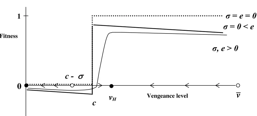
First consider the case σ = e = 0, where v is perfectly perceived and behavior is noiseless.
Recall that in this case the short run equilibrium (N, D) with payoffw= 0 prevails forv≤c, and
(T, C) with w= 1 prevails for v≥c. Thus w(v; 0,0) is the unit step function atv =c, shown as
the dotted line in Figure 3.
———–fig 3 about here———–
With behavioral but no perceptual noise, e >0 =σ, more vengeful types incur a greater cost
when punishment is called for. The bold solid line in Figure 3 shows that now Self’s fitness function
slopes downward at approximate rate −e. Finally, with perceptual noise also present, σ >0, the
sharp step at v = c is smoothed out. Figure 3 shows two local fitness maxima for Self, one at
v = 0 and the other atv = vH > c, when σ and e are both small and positive. The underlying
calculations are collected in subsection 4 of the Appendix.
The fitness functionwdefines a one-dimensional landscape in which evolution pushes the
evolv-ing traitv uphill along the fitness gradient.11 Figure 3 therefore suggests that we will end up with
some fractionx of the Self population with vengeance nearvH > c and the remaining (1−x) with
vengeance near v = 0. The fractions represent the arbitrary portions of the population initially
above and below the fitness minimum (near c−σ).
4
Perfect Bayesian Equilibrium
The implication of the preceding discussion in the previous section is that we don’t need to consider
all possible distributions over a continuum of vengeance types. The equilibrium distributions will
have support on just two points, one at v = 0 and the other at some specific vH > c, fixed in
the short run but variable in the long run. With just two types, we streamline the short run
analysis (at a slight loss of generality) by focusing on the misperception probabilities rather than
the entire error distribution. Therefore we define perception as a binary variable s, with s = 1
11
As its title suggests, the present paper does not specify evolutionary dynamics. However, dynamical intuition
will help motivate the formal definition of EPBE presented below. We therefore note that continuous movement up
the fitness gradient has well established antecedents, e.g., Wright (1949), Eshel (1983) and Kauffman (1993). Such
landscape dynamics (Friedman, 2005) are quite distinct conceptually and formally from mutations in a discrete type
denoting the perception that Self is vengeful, and s = 0 denoting the perception that Self is not
vengeful. It is convenient (but not essential) to assume equal misperception probabilities and write
a= Pr[s= 0|v=vH] = Pr[s= 1|v= 0].
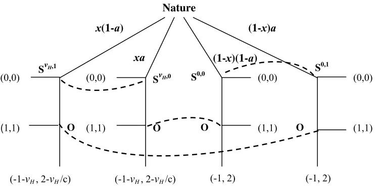
———–fig 4 about here———–
Figure 4 shows the game tree. Nature chooses Self’s true preference parameter as v = 0
(unvengeful) with probability 1−x, or as v = vH > c (vengeful) with probabilityx. Nature also
independently chooses Other’s perception as correct (s = 0 for v = 0, or s= 1 for v = vH) with
probability 1−a, or incorrect with probabilitya∈[0,1/2).Self knows her own preference but not
the realized perception, and Other knows the perception but not the true preference.
Self’s “pure” strategy set is denoted {NN, NT, TN and TT}, where XY means the unvengeful
type tries to play X and the vengeful type tries to play Y. To spell this out, the space of mixed
strategies is the unit square with corners at the pure strategies when there are no trembles. With
trembles e ≥ 0, Self’s strategy space shrinks to the smaller square [e,1−e]×[e,1−e], and a
corner strategy such as NT means that that N and T are actually played with probability 1−eby
respectively the unvengeful and vengeful type Self. Similarly, Other’s “pure” strategy set is{DD,
DC, CD and CC}, where now XY stands for the strategy ‘play X if s = 0 and play Y if s = 1.’
Here ”play” means to actually play with maximal probability 1−e.Thus Other’s strategy space is
also [e,1−e]×[e,1−e]. The payoffs shown in Figure 4 are the same as in the reduced Trust game
of Figure 2C.
The relevant equilibrium concept is perfect Bayesian equilibrium, PBE (e.g., Fudenberg and
Tirole, 1991, chapter 8), suitably phrased to deal with large populations and explicit trembles.
PBE requires all players to optimize given beliefs, and requires that beliefs are Bayesian
poste-rior probabilities obtained from perceptions, observed actions, and pposte-rior information on the type
proportions.
What sort of PBE might exist? The first candidate is a separating equilibrium, call it SEP, in
which Other plays DC and Self plays NT. Other prominent candidates are GP, the “good pooling”
PBE in which Self plays TT and Other plays CC, and the “bad pooling ” equilibrium BP = (NN,
DD). In testing for any of these equilibria, the key conditions arise from Other’s decision problem
after a noisy perception. Other compares the expectation of the D payoff 2−v/cto the C payoff 1.
This comparison immediately leads to the rule: play D if E(v|s)≤c, or play C if E(v|s) ≥c. To
illustrate, consider an s= 0 perception when Self plays NT. The perception is erroneous precisely
when a vH type actually chooses T (i.e., doesn’t tremble) and Other misperceives, which happens
with probabilityx(1−e)a. The perception is correct precisely when av= 0 type trembles to T and
calculation now shows that the critical posterior expectation E(v|s= 0) =c corresponds to prior
probability (or population fraction) xs = 1/(1 + ( a 1−a)(1
−e e )(vH
−c
c )). Hence the rule states that
Other should play D when observings= 0 ifx≤xs.Using the log odds function L(y) = ln(1−y y ),
this necessary condition for SEP can be rewrittenL(x)≥L(xs) =−L(a) +L(e) +L(c/vH).
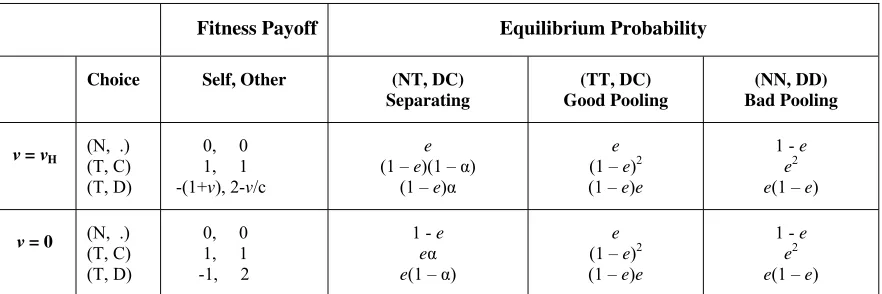
———–table 1 about here———–
Using Table 1, the reader can perform very similar calculations for other cases (s= 1
percep-tions and Self strategies TT and NN) to obtain bounds on Other’s best responses in terms of the
population fractions x or their log odds. Combining them with straightforward computations of
Self’s best responses leads to necessary and sufficient conditions for the existence of the three pure
strategy PBEs.
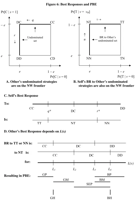
Straightforward computations show that Other strategy CD is dominated and that Self strategy
TN is never a best response to Other’s undominated strategies, so only strategies on the Northwest
frontier of the strategy spaces need be considered in candidate PBEs. As shown in Figure 5, SEP
and BP exist over overlapping ranges in the prevalence x of vengeful types, and there is a gap
between these and the range where GP exists.
————–fig 5 about here——
There are also mixed PBEs.12 The best response correspondences show that there is some mix
q∗ ∈ [0,1] of DC and CC that makes Self indifferent between TT and NT. We have a candidate
mixed PBE if there is also some mix t∗
(x) ∈ [0,1] of TT and NT that makes Other indifferent
between DC and CC. It turns out that the profile (t∗(x)T T + (1−t∗(x))N T, q∗DC+ (1−q∗)CC)
is a PBE, call it the Good Mix (GM), precisely whenx lies in the gap.
Are there any other mixed PBEs? The same logic points to one other possibility. Consider
(u∗
(x)N T + (1−u∗
(x))N N, r∗
DD+ (1−r∗
)DC), wherer∗
∈[0,1] makes Self indifferent between
NN and NT, andu∗(x)∈[0,1] makes Other indifferent between DC and DD. This Bad Mix (BM),
as we shall call it, turns out to be a PBE wheneverx lies in the range overlap for the BP and the
SEP PBEs.
The best response correspondences permit no other PBEs over a nontrivial range ofx. They do
produce other PBEs at two isolated points. When L(x) = L(c/vH)−L(a), both CC and DC are
best responses to TT, and TT is a best response to qDC+ (1−q)CC as long asq ∈[0, q∗]. Hence
at this point, there is a continuum of PBEs, call them Good Hybrids, that vary only in Other’s
mixing probabilityq. Finally, whereL(x) =L(c/vH) +L(e) +L(a), we have the Bad Hybrids (BH)
(NT,rDD+ (1-r)DC) for r∈[r∗
,1]. Proposition 1 characterizes all the PBEs.
Proposition 1. Given perceptions with error rate a and choices with tremble rate e, and
12
given types v = 0 and v =vH > c constituting respectively Self population fractions (1−x) and
x∈(0,1),assume that 0< a, e <1/2 andα=a+e−2ae≤1/(2 +vH). The complete set of PBE
consists of:
1. the GP family (TT, CC) forL(x)≤L(c/vH)−L(a);
2. the SEP family (NT, DC) for L(c/vH) +L(e)−L(a)≤L(x)≤L(c/vH) +L(e) +L(a);
3. the BP family (NN, DD) forL(x)≥L(c/vH) +L(a);
4. the GM family (t∗(x)TT+(1-t∗(x))NT, q∗DC+(1-q∗)CC) for L(c/v
H) − L(a) ≤ L(x) ≤
L(c/vH) +L(e)−L(a);
5. the BM family (u∗
(x)NT+(1-u∗
(x))NN, r∗
DD+(1-r∗
)DC) for L(c/vH) + L(a) ≤ L(x) ≤
L(c/vH) +L(e) +L(a);
6. the GH family (TT,qDC+(1-q)CC), forq ∈[0, q∗], at the point whereL(x) =L(c/v
H)−L(a);
and
7. the BH family (NT, rDD+(1-r)DC) for r ∈ [r∗,1], at the point where L(x) = L(c/v H) +
L(e) +L(a).
The proof, in the Appendix, includes formulas for q∗
, r∗
, t∗
and u∗
.
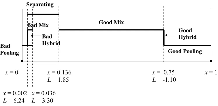
A numerical example will help fix ideas. Set the marginal punishment cost at c= 0.5 and the
vengeful type’s preferred punishment expenditure atvH = 2.0.Set the tremble rate ate= 0.05 and
the misperception rate at a= 0.10.As shown in Figure 5, for sufficiently small proportions of the
vengeful type (L(x)≥3.30 orx≤0.036) we have a Bad Pooling equilibrium: both types of Self try
to opt out and Other tries to defect regardless of perception. For an overlapping range of vengeful
type proportions (L(x)∈[1.85,6.24] or x∈[0.002,0.136]) we have the Separating equilibrium. In
the overlap x ∈ [0.036,0.136], there is also the Bad Mix PBE. No pure strategy PBE exists (just
the Good Mix PBE, for which q∗ = 5/9 and t∗(x) ≈ .35 x
1−x −.06) for higher values of x until
we reach x = 0.75, after which point we have the Good Pooling equilibrium. The Good Hybrid
equilibrium exists atx=0.75 forq∈[0,5/9], and the Bad Hybrid equilibrium exists atx=0.002 for
r∈[70/81,1].
5
Evolutionary Perfect Bayesian Equilibrium
The numerical example spotlights an evolutionary problem. In the separating PBE, the vengeful
of evolution, the fraction x of vengeful types should increase. But the separating PBE disappears
when x gets above .136. The same is true for the GM equilibrium: the vengeful types have fitness
0.665 while the unvengeful types have fitness 0, so again x should increase past the point (here
0.75) where the equilibrium disappears. However, whenx > .75, we have only the GP equilibrium.
Now the unvengeful type is fitter (0.855) than the vengeful type (0.760), soxshould decrease until
it falls below .75 and the GP equilibrium disappears. None of these equilibria seems stable in the
long run.
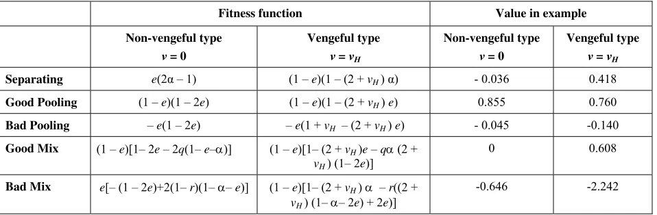
———–table 2 about here———–
The evolutionary problem is not due to an unfortunate parameter choice in the numerical
example. In the separating PBE, the vengeful type always achieves positive fitness; otherwise
she would not try to play T. The unvengeful type always has negative fitness in this equilibrium
because, with observational error rate a < 1/2, the payoff -1 is more frequent than +1. (See
Table 2 for the general fitness expressions.) Hence evolutionary forces will always increase x in
the separating PBE. In the GP equilibrium, the vengeful type always has lower fitness because of
the extra cost (1−e)vHe of reacting to Other’s trembles, so evolutionary forces will decrease x.
Unvengeful types in the GM equilibrium always have fitness zero, and vengeful types always have
nonnegative fitness. Once again,x will tend to increase until the equilibrium disappears. It seems
that evolution undermines perfect Bayesian equilibrium.
5.1 Equal Fitness Principle
The problem is not due just to the peculiarities of our noisy trust game. Games of incomplete
information generally have multiple types, and numerous mechanisms tend to increase the
preva-lence of high payoff types relative to low payoff types. For example, in an industry where firms
with high quality products compete with those with low quality, one expects the market share of
the less profitable type of firms to decrease over time because such firms expand less rapidly or
exit, or switch types. As another example, a type of worker with lower full compensation (earnings,
benefits and perks net of effort cost and opportunity cost) should become less prevalent due to
earlier retirements, lower accession rates, etc.
The point is that payoffs should be equal across surviving types in long run equilibrium. In this
context, PBE (or any standard refinement) is a short run equilibrium concept, while in the long run
the types and their relative prevalence should adjust so that only those types with highest payoff
remain. This is precisely the “survival of the fittest” principle of evolutionary theory. It is also
the textbook distinction between short run and long run competitive equilibrium. The Appendix
extensive form games of incomplete information.
Definition. An evolutionary perfect Bayesian equilibrium (EPBE) is a PBE distribution over
type-contingent strategy profiles such that in each population all types in the support of the
dis-tribution achieve equal and maximal expected fitness.
We now develop the EPBE concept specifically for our noisy trust game with endogenous values
for the vengeful typevH, its prevalencexand the perceptual error ratea. In EPBE,vH maximizes
fitness over an appropriate space of types, which we shall take to be the closed interval [0, vmax].
The idea is that within broad limits, social (and perhaps genetic) forces shape Self’s emotional
response to violation of trust. We assumevmax>0 is large enough not to be a binding constraint;
see Friedman and Singh (2004a) for a supporting discussion. In general one considers a distribution
or measure over the space of types, but (for reasons discussed above in connection with Figure 2)
the relevant distributions in the noisy trust game have support on at most two points, v = 0 and
v=vH < vmax.
A fitness maximizing value vH > 0 will be characterized by a marginal balance between two
opposing effects. When vengefulness increases,
Perception Effect: Other is more likely to perceive v > c (ors= 1), and hence is more likely to
choose C, enhancing Self’s fitness. However,
Cost Effect: when Other chooses D (either intentionally or via a tremble), Self will incur greater
cost to punish him, reducing Self’s fitness.
The cost effect can be derived from model elements used in the PBE analysis, but the perception
effect cannot. Extremely vengeful types should be easier than slightly vengeful types to distinguish
from v = 0 types, so the misperception probability a must be endogenized. For convenience
we simply postulate a = A(v),13 where A is a smooth, positive and decreasing function, with
A(0) = 1/2 andA(v)→0 asv→ ∞. Thus the types cannot be distinguished when vengefulness is
negligible, and can be distinguished perfectly in the limit as the vengefulness becomes extreme.
Crisp results require a parametric form for the perception technology A.Our choice is a simple
Gaussian function with precision parameterk >0,
A(v) = 0.5 exp(−kv2),so A′
=−2kvA. (1)
Besides the perception technology A(or precision parameter k >0), we retain only two
exoge-nous parameters: the marginal punishment cost parameter c >0 and the tremble rate e∈[0,1/2).
13
In principle, one could deriveAfrom the underlying distribution of perception errorsy. In practice, estimating
the error distribution is unlikely to be as useful as estimatingA directly. Note that the argument in Appendix 7.4
We continue to assume error symmetry for simplicity.
Characterizing EBPE for the noisy trust game comes down to the following conditions. Given
the exogenous parameters, find endogenous values fora, vH andx such that
1. There is a PBE strategy profile for the exogenous parameters c and e and the endogenous
values a, vH,andx.
2. The misperception rate is a=A(vH).
3. The preference parametervH maximizes Self’s expected fitness given Other’s PBE strategy.
Formally,
vH = arg max v∈[c,vmax
]{EqW
S(v|A(v), e)}, (2)
where EqWS is the maximal expected fitness Self can attain in the constrained strategy set
[e,1−e], given Other’s q-mixed strategy. The cost effect is captured in the argumentv and
the perception effect is captured in the conditioning variable A(v).
4. If 0< x <1 then the equal fitness principle implies that the unvengeful type Self achieves the
same maximal expected fitness as the vengeful type, given Other’s PBE strategy. Formally,
EqWS(0|A(0), e) =EqWS(vH|A(vH), e). (3)
That is, the strategy mixq employed by Other must equalize payoffs between unvengeful and
vengeful Selfs.
5. If 0 < q < 1 then the equal fitness principle requires that both surviving types of Other
achieve equal fitness, i.e.,
ExWO(CC|a, e) =ExWO(DC|a, e). (4)
One must also check that the extinct types of Other (DD and CD, and also DC when q= 0
and CC when q= 1) achieve no higher fitness.
5.2 Results
What sort of PBE might survive the EPBE refinement? The discussion at the beginning of this
section showed that the equal fitness principle fails for the SEP and GP families of PBE; specifically
condition 4 fails except at GP withx= 1, where condition 3 fails. The discussion also showed that
the GM family is an unlikely habitat for EPBEs; the Appendix rules it out.
Clearly the BP family contains a trivial EPBE. The family exists when vengeful types are so
are always fitter because trembles hurt them less. Hence the vengeful types become extinct, i.e.,
x → 0, so the only possible BP candidate for EPBE is at the extreme, x = 0. It indeed is an
EPBE: condition 1 holds because we are already working with a PBE, condition 3 holds because
v= 0 uniquely maximizes Self’s fitness, and conditions 2, 4 and 5 are moot. In this EPBE (except
for double trembles) there are no mutual gains.
When might there be an efficient EPBE, one that supports mutual gains in the noisy trust
game? The BM and BH families are unlikely habitats, again ruled out in the Appendix. The
remaining family, Good Hybrid (GH), seems more promising because it allows both vengeful and
unvengeful Selfs to achieve positive fitness, sometimes higher for the vengeful and sometimes higher
for unvengeful. The GH strategy profiles are (TT, qDC + (1-q)CC).
Our main result is that such an efficient EPBE does exist and is unique over a wide range of
the exogenous parameters. The upper bound on the tremble rate is an increasing function ˆe(k) of
the precision parameterk, derived in the Appendix. This bound is approximately 0.23 (i.e., players
might tremble a bit more than once in five tries) whenk= 0.5 as in the unit Normal distribution,
and it is about 0.13 fork= 0.1.
Proposition 2. Given marginal punishment costc∈(0,1), behavioral error ratee∈(0,ˆe(k)),
and perception technology (1) with precision parameterk∈(0,0.6), there is a unique efficient (Good
Hybrid) EPBE whose characteristics (vH, a, q, x) depend smoothly on the exogenous parameters.
There is only one other EPBE in the noisy trust game: the trivial (Bad Pooling) EPBE with
proportionx= 0 of vengeful types. It exists for all perception technologies, all marginal punishment
costsc >0, and all behavioral error rates e∈(0,1/2).
The parameter k is bounded above by ¯k≈0.612; at higher values, the second order condition
forvH fails. A finite value ofvmax creates a lower bound on k; for examplev < vmax = 10 implies
k >0.028. The proposition restricts parameter c to its natural interval (0,1). Higher values of c
(for which Self’s fitness reduction is larger than Other’s) can tighten the upper bound onk due to
the constraintvH > c. For example, when c= 2 the upper bound is near k= 0.3.
The proof appears in the Appendix. It is constructive, and proceeds by writing explicit versions
of the last three equations, solving them in terms of the exogenous parameters, and checking the
relevant side conditions. It turns out that the equilibrium valuesvH =v∗(k) anda=a∗(k) depend
on k but are independent of e and c, while q = Q(e, k) is independent of c, and x = X(c, k) is
independent ofe.
Some of the comparative statics for the efficient EPBE are intuitive and others take a little
effect, the equilibrium level of vengeance declines as perceptions become more precise. Perhaps
surprisingly, a∗ is increasing in k, that is, the equilibrium observational error rate goes up as the
precision increases. It turns out that the indirect effect viav∗
(k) dominates the direct effect of k.
How about the probability with which Other attends to perceptions? Q(e, k) increases in the
tremble rateeas a consequence of the Self’s indifference condition (3), and decreases in the precision
of perceptions, k. Finally, the equilibrium fraction X(c, k) of vengeful Selfs increases in the cost
of punishmentcas a consequence of the Other’s indifference condition (4). However, the precision
parameterk can have either a positive or negative effect on X depending on the level ofc.
6
Discussion
We may summarize the argument as follows. Economists need to come to grips with human motives
such as vengeance. Since vengeance generally reduces own material payoff or fitness, its persistence
is an evolutionary puzzle. We therefore construct a model in which a taste for vengeance survives in
a long run evolutionary equilibrium. The model uses emotional state dependent utility components
(ESDUCs) to represent such motives. The presence of ESDUCs is the proximate answer to the
question of why individuals may want to harm (or help) others. However, the deeper questions
of why specific ESDUCs exist and how they survive requires an analysis of their indirect fitness
consequences. Studying vengeance is just one (interesting and complicated) application of the
indirect evolutionary approach.
Our answer to the evolutionary puzzle proceeds in three stages. First, we construct a simple but
representative situation in which ESDUCs matter, viz., a noisy version of the Trust game played
in large unstructured groups. Second, we compute all perfect Bayesian equilibria (PBE). We note
that different types of individuals (vengeful or not) have different fitness in most PBE, leaving
room for evolutionary pressures to operate. The third stage, therefore, is to introduce a new long
run equilibrium concept called evolutionary PBE, which allows adjustment in the proportion of
vengeful types, as well as the intensity of their vengefulness. We characterize the unique efficient
EPBE for a wide domain of parameter values.
The conclusions are fairly robust within the context of the noisy Trust game. The argument can
accommodate more general specifications of the payoffs, the perception technology, the punishment
technology and preferences, and asymmetric perception errors. The Appendix shows that the
expressions become much messier but the qualitative results are unchanged.
dynami-cally stable? The answer may depend the specific form of adjustment dynamics.14 Friedman and
Singh (2004a) suggests that short run dynamics enforcing PBE are entirely cultural (e.g., imitation
or belief learning), and that the longer run dynamics enforcing EPBE also are mostly cultural
(e.g. family moral codes) with some genetic components (e.g., capacity for anger). A relatively
uncontroversial form of group selection (Wright’s shifting balance) may promote convergence to the
efficient EPBE. Adjustment dynamics surely are an important area for future work.
A second question concerns the trivial EPBE: how can one get a critical mass to escape it? Put
more simply, in the context of the basic Trust game in Figure 1, how can one get v > c starting
from v = 0? Friedman and Singh (2004b) suggests a possible answer to this threshold problem.
Subthreshold v < c is not adaptive in a large population, but in small groups it works together
with the discount factorδ to increase fitness. Thus positive values ofvcould get started in smaller
groups and eventually become advantageous in larger groups.
Third, which remaining parameters can be endogenized? Keeping punishment technology c
constant (or doing comparative statics exercises for c) seems to make sense. The tremble rate
parameter e trades off trivially against the endogenous probability q that Other attends to the
perception, as can be seen from equations (7) and (10) in the Appendix. However, there is every
reason to take seriously the evolution of perception technology. Obviously Others who evolve a
better perception technology (e.g., a lower value of k) would receive a fitness boost. On the other
hand, so would a mutant Self with true vengeance parameter v = 0 who could somehow mimic
the vengeful type, in effect increasing k. Friedman and Singh (2004b) refer to this possibility as
the Viceroy problem, a reference to toxic Monarch butterflies that correspond to vengeful types
and their mimics known as Viceroys. That paper sketches an elaborate solution to the problem
that involves interactions within and across small groups, but the issue remains open for large
unstructured populations.
How might the ideas extend to more general classes of games? After all, people play many
different social games, not just the noisy Trust game.15 For example, consider the famous
Ultima-tum game. The first mover proposes a division of a fixed pie. A second mover with v = 0 will
accept any proposal that gives him a positive payoff, but in most experiments the second mover
often rejects small offers, giving both players zero payoff. Cox et al (2007) estimate parameters
14
The dynamic analysis is complex since we have a continuum of potential types. Our current conjecture is that for
all sensible dynamics the trivial (and inefficient) EPBE will have an open basin of attraction, and that the efficient
EPBE will be stable in the same sense for some dynamics and for other sensible dynamics will be neutrally stable
(e.g., will have a one dimensional stable manifold and a two dimensional center manifold).
15
Our methods apply directly to any stable mix of games, and comparative statics apply to small one-time shifts
that translate to v > 0, but they do not consider equilibrium. It is reasonable to conjecture that
a noisy version of the Ultimatum game supports two EPBE: a trivial EPBE with only v = 0 and
greedy proposals, and an equitable EPBE with a mix of vengeful and unvengeful second movers
and with more generous proposals.
We do not claim existence and uniqueness of nontrivial EPBE in great generality. In our Trust
game (and also, it would seem, in a noisy Ultimatum game) the payoff ordering of vengeful and
unvengeful types differs in different PBE, and this was the key to obtaining the nontrivial EPBE.
We suspect that only trivial EPBE can exist when the same type in a given population has the
highest payoff in every PBE, or when there are not enough margins for evolutionary adjustment.
As for non-uniqueness, Abreu and Sethi (2003) obtain a continuum of EPBE in a bargaining model
with wide classes of behavioral types. On the other hand, Friedman and Singh (2004a) study a
simultaneous move social dilemma and obtain an efficient equilibrium, implicitly an EPBE with
only one particular vengeful type. The questions of EPBE existence, uniqueness and efficiency
remain open for general classes of games.
To conclude, the present paper combines two ideas, each of which we believe has widespread
applicability independent of the other. Emotional state dependent utility components (ESDUCs)
offer a tractable and flexible way to model other-regarding preferences, and can address several
important issues in behavioral economics. In particular, the vengeful components emphasized in
the present paper may help give new insights into ”irrational” conflicts ranging from employment
relations to international struggles. Friendly components likewise may give insight into behavior
within the family and firm, and into the dynamics of charitable giving and social capital.
The second idea is evolutionary Perfect Bayesian equilibrium (EPBE). We wrote a general
verbal definition and worked it out explicitly for a particular (and not especially simple) game of
incomplete information. The Appendix concludes with a more general definition and remarks. We
believe that EPBE is an appropriate characterization of long run behavior when there are multiple
potential ”types” and some opportunity for entry, exit and/or switching among types. EPBE
endogenizes the set of types and their proportions, key variables that otherwise must be specified
7
Appendix. Mathematical Details.
7.1 Proof of Proposition 1
Letq∗ = 1/(2−2a)∈(1/2,1) and define t∗(x)∈(0,1) as the solution to
(1−c/vH
c/vH
)( x
1−x) =t(
1−a
a ) + (1−t)(
1−a a )(
e
1−e). (5)
Also, letr∗ = [1 +v
H −e(2 +vH)]/[(1−a)(1−2e)(2 +vH)] =q∗(1+v2+vHH −e)/(21 −e)∈(q∗,1) and
defineu∗
(x)∈(0,1) as the solution to
( c/vH 1−c/vH
)(1−x
x ) = (1−u)(
1−a a ) +u(
1−a a )(
1−e
e ). (6)
To check for all PBE we map out the best response correspondences (building in Bayesian
updating) and look for mutually consistent profiles. We proceed stepwise.
Step 1. Confirm that CD is dominated. Recall from the payoff structure that Other is indifferent
between C and D iff E(v|s) =c, and strictly prefers C (D) if E(v|s) >(<)c. It follows that DD
dominates CD if c > E(v|s = 0), and that CC dominates CD ifc < E(v|s = 1). At least one of
these two cases always holds sinceE(v|s= 1)> E(v|s= 0), establishing the claim. ♦
Step 2. The only undominated Self strategies in Figure 6A are those on the NW frontier. Any
other strategyY can be written as a convex combination of CD and a NW frontier strategy, since
the set is the convex hull of its four corners, and the other three corners are contained in the NW
frontier. But step 1 shows that CD and hence Y is dominated. ♦
————–Figure 6 about here————
Step 3. TN is not a best response to any undominated strategy of Self. Direct computation
shows that the best responses are as in Figure 6C: TT along the portion of the N frontier (convex
combos of CC and DC) east of q∗, NT around the NW corner, and NN for the portion of the W
frontier south of r∗
.
To spell it out, we show explicitly that NT is always the best response to DC, as is TT to CC,
given the hypotheses 0< a, e <1/2 andα =a+e−2ae≤1/(2 +vH). Suppose that Other will play
DC. Then Self withv=vH will face D with probabilityα= (1−e)a+e(1−a) =a+e−2ae when
playing T. A simple calculation shows that Self’s expected payoff is nonnegative (and therefore
she will indeed try to play T) as long as α ≤ 1/(2 +v), which holds by hypothesis. Self with
v = 0 will face D with probability 1−α when playing T; and she will avoid doing so as long as
α≤1/(2 +v) = 1/2,a redundant condition. Hence NT is indeed the best reply to DC. If instead
Other plays CC, the condition ensuring that Self indeed wants to play T is the same as before,
The q∗
-mix of DC and CC that makes Self indifferent between NT and TT is precisely the mix
that gives unvengeful Self zero expected payoff when actually choosing T, because the actual N
payoff is also (always) 0. This condition is 0 = EqWS(T|v = 0) ≡ 1(1−γ)−1γ, or γ = 1/2,
where γ is the probability that Other actually chooses D when unvengeful Self chooses T. There
are three ways this can happen: Other ignoressbut trembles, with probabilityγ1 = (1−q)e; Other
incorrectly perceivess= 1 and trembles, with probability γ2 =qae; and Other correctly perceives
s= 0 and doesn’t tremble, with probability γ3 =q(1−a)(1−e). So the condition is 1/2 = γ =
γ1+γ2+γ3 =e+q(1−2e)(1−a). The solution is indeedq∗ = 1/(2−2a),and is clearly unique.
It follows that NT (resp. TT) is Self’s best response toqDC + (1-q)CC for q ∈[0,1] larger (resp.
smaller) thanq∗
.
By a very similar argument, one verifies that r∗ = q∗(1+vH
2+vH −e)/( 1
2 −e) makes vengeful Self
indifferent between N and T in response tor-mixes of DD and DC. (The condition is that vengeful
Self obtains payoff zero from T, or 0 =−(1+v)[(1−e)−r(1−a)(1−2e)]+[1−(1−e)+r(1−a)(1−2e)],
with root r∗
.) Again, it follows that NN (resp. NT) is Self’s best response torDD + (1-r)DC for
r∈[0,1] larger (resp. smaller) thanr∗. ♦
Thus any mutual best response involves only the NW frontier strategies, TT-NT-NN for Self
and CC-DC-DD for Other. The proof will be complete after we check all combinations for mutual
consistency.
To streamline notation, letL1 =L(c/vH)−L(a);L2 =L(c/vH)−L(a) +L(e);L3=L(c/vH) +
L(a); andL4 =L(c/vH) +L(a) +L(e). We have Li < Li+1 becauseL(a) andL(e) are positive for
a, e <1/2.
Step 4. Suppose first that Other perceivess= 0 when Self plays NT. Recall that in this case the
perception is erroneous with probability x(1−e)aand is correct with probability (1−x)e(1−a).
Hence by Bayes Theorem c=E(v|s= 0) = vHPr[v=vH|s= 0] + 0 =vH[x(1−e)a/(x(1−e)a+
(1−x)e(1−a))].Cross-multiply, divide both sides by ca(1−e)(1−x) and collect terms to obtain
1−x
x = (1−aa)(1 −e e )(
1−c/vH
c/vH ).RecallL(y) = ln( 1−y
y ) for y∈(0,1), so ln( y
1−y) =−L(y).Hence Other
is indifferent after seeings= 0 whenL(x) =−L(a) +L(e) +L(c/vH),and prefers D when the prior
odds L(x) that v =vH are longer. When Self plays NT, Other will correctly perceive s= 1 with
probabilityx(1−e)(1−a) and incorrectly perceive it (i.e., whenv= 0) with probability (1−x)ea.
Algebra similar to thes= 0 case shows thatL(x)≤L(c/vH) +L(e) +L(a) now motivates Other
to play C. Note thatL(a) is positive sincea <1/2. Hence DC is Other’s best response to NT over
the relevantx-range. If Self plays TT and
s= 0, the expression (1−x)e(1−a) for NT is replaced by (1−x)(1−e)(1−a) in the Bayesian
that Other wants to play C even whens= 0 iffL(x)≤L(c/vH)−L(a). That is, CC here is a best
response to TT.
These computations are summarized in the first two lines of Figure 6D. The top line indicates
that the unique best response to TT (or to NN!) is CC forL(x)< L1, is DC for L1 < L(x) < L3,
and is DD for L(x) > L3; at L1 the best responses are CC and DC (and convex combinations),
and atL3 the best responses are DD and DC (and convex combinations). Likewise, the second line
indicates that the unique best responses to NT are CC for L(x) < L2, DC for L2 < L(x) < L4,
and DD for L(x) > L4; at L2 the best responses are all convex combinations of CC and DC, and
atL4 they are all convex combinations of DD and DC.♦
Step 5. We now examine every Self strategy that could be part of a PBE, find all best responses
by Other, and check for mutual consistency. Begin with TT. For L(x) < L1, the unique best
response is CC, and TT is its best response, so we see that the GP family (TT, CC) is a PBE, and
that there is no other candidate in this case. ForL(x) =L1, step 4 told us that the best responses
to TT are convex combinations of DC and CC. Step 3 told us that TT is a best response to the
convex combination qDC+ (1-q)CC iff q ∈ [0, q∗], and is never a best response to DD or DC (or
convex combinations). Hence the only PBE where Self plays TT and L(x) = L1 consist of the
q ∈[0, q∗] mixes, i.e., the GH family. When L(x)> L
1, the best response to TT is DD or DC, to
which TT is never a best response. Hence there are no other PBE profiles where Self plays TT.♦
Step 6. Now consider strict mixes of TT and NT. By Figure 6D, the unique best response is
CC for L(x) < L1, but NT can’t be a best response to CC so no such PBE is possible here. For
L(x)> L2 the best responses are DC and DD, neither of which admits TT as a best response, so
again no such PBE is possible. But for anyxsuch thatL1 ≤L(x)≤L2 we can construct a unique
PBE, which takes the Good Mix form (t∗
(x)TT+(1-t∗
(x))NT, q∗
DC+(1-q∗
)CC). The construction
proceeds as follows.
Recall from step 3 that only q∗
= 1/(2−2a) mixes of DC and CC allow strict mixes of TT and
NT as best responses. Hence it suffices to find t∗(x)∈(0,1) such that convex combinations of DC
and CC are best responses to the the t∗
mix of TT and NT. That is,t∗
(x) makes Other indifferent
between N and T when s= 0. The condition is c= E(v|s = 0) =vHβ, whereβ is the posterior
probability that Self is vengeful. Thusβ =x(1−e)a/η, whereη is the unconditional probability of
Other seeings= 0, which now can happen in three different ways. The first way (also represented
in the numerator) is that a vengeful Self doesn’t tremble but is misperceived: η1 =x(1−e)a. The
second way is that an unvengeful Self tries to play T, doesn’t tremble, and is correctly perceived:
η2 = t(1−x)(1−e)(1−a). The last way is that an unvengeful Self tries to play N, trembles,
(after cross-multiplying) is η1vH/c = η1+η2 +η3. Collecting the η1 terms and dividing through
by a(1−x)(1−e) we obtain equation (5). Observe that the RHS of (5) is strictly increasing in t
since 0< e <1/2. Whent= 0 in (5) we obtainL(x) =L2, and when t= 1 we obtain L(x) =L1.
Hence for intermediate values of x, which satisfy the given inequalities L1 ≤L(x)≤L2 we obtain
from (5) a unique t∗
∈[0,1] that makes Other indifferent between C and D whens= 0.♦
Step 7. Now consider pure NT. The argument has the same structure as step 5. We confirm
that forxsuch thatL2≤L(x)< L4, the SEP family (NT, DC) is the only PBE in which Self plays
NT. ForL(x) =L4, the best responses to NT are convex combinations of DC and DD, and NT is a
best response torDD + (1-r)DC iffr ∈[r∗,1]. NT is never a best response to convex combinations
of CC and DC. Hence we pick up the BH family. When Other best responds to NT with DD (as
will happen if L(x) > L4), then Self’s best response is not NT but rather NN. Likewise, when
Other best responds to NT with CC (as will happen ifL(x)< L2), then Self’s best response is not
NT but rather TT. In neither case can we have a PBE of the desired form.♦
Step 8. Now consider strict mixes of NN and NT. The argument has the same structure as
step 6. Self will play such a mix in mutual best response only if L3 ≤L(x)≤L4 and Other plays
the r∗
mix of DC and DD. The mix of NN and NT that allows Other to mix DC and DD must
satisfy c = E(v|s = 1) = vH(κ1+κ2)/(κ1+κ2+κ3), where κ1 =xu(1−a)(1−e) for correctly
perceived vengeful Self not trembling, κ2 = x(1−u)(1−a)e for correctly perceived vengeful Self
trembling, κ3 = (1−x)ae) for incorrectly perceived unvengeful Self trembling. The expression can
be rewritten to obtain (6). Hence we obtain the BM family and no other PBEs.♦
Step 9. Finally consider pure NN. ForL(x)> L3, DD is the unique best response, and NN is of
course the best response to DD, so we see that the BP family (NN, DD) is a PBE, and that there
is no other candidate in this case. ForL(x) =L3, the only candidates are the BP and the extreme
BM with u= 0; both are already picked up. When L(x) < L3, the best response to NN is CC or
DC, for which NN is never a best response. Hence there are no other PBE profiles where Self plays
NN. ♦
Step 10. We picked up the GP and GH families at step 5, the GM family at step 6, the SEP
and BH families at step 7, the BM family at step 8, and the BP family at step 9. Since we now
have looked at all possible equilibrium profiles, the proof is complete.♦
7.2 Proof of Proposition 2 and comparative statics
For convenience, the derivations of comparative statics are included in this proof. The Proposition
applies to a parameter domain defined by the functions R(k) = (kv(2 +v)− 12) exp(−kv2) and
ˆ
aare specific functions (derived below) of konly.
The first and most laborious step in the proof is to derive vH for a given k. Recall that
the Good Hybrid strategy profile is (TT, qDC+(1-q)CC), so the probabilities in Table 1 give
the fitness function EqWS(v) = (1−e)[q(1−α −(1 + v)α) + (1−q)((1 −e) −(1 + v)e)] =
(1−e)[1−(2 +v)e−qa(2 +v)(1−2e)]. The first order condition (FOC) 0 =dEqWS/dv for the
maximization problem (2) simplifies slightly to 0 =−e−qA′(2+v)(1−2e)−qa(1−2e) or, separating
variables,
[ e 1−2e]q
−1=−(2 +v)A′
−a. (7)
The second order condition is (2 +v)A′′
+ 2A′
≥0. Substituting in theA′
expressions from (1), the
FOC is
[ e 1−2e]q
−1= [2kv(2 +v)−1]a= (kv(2 +v)− 1
2) exp(−kv
2) (8)
and the SOC is
kv3+ 2kv2−3
2v−1≥0. (9)
Equation (3) says that vengeful and unvengeful type Selfs coexist in the EPBE because they
have equal fitness. Recall that EqWS(v) = (1−e)[1−(2 +v)e−qa(2 +v)(1−2e)].Recall also
that we are looking for an EPBE in which even the unvengeful try to play T, so EqWS(0) =
(1−e)[q(α−(1−α)) + (1−q)((1−e)−e)] = (1−e)[1−2e−q(2−2a−4e+ 4ae)]. Thus (3)
reduces tove=q[2(1−2α)−av(1−2e)] =q(1−2e)[2−a(4 +v)].Separating variables again, we
obtain
[ e 1−2e]q
−1= (2−a(4 +v))/v. (10)
Note that (8) and (10) have the same left hand side. Equating the right hand sides, we get
2kv(2 +v)a−a= (2−4a)/v−aor
kv3+ 2kv2+ 2 = 2 exp(kv2) = 1/a. (11)
This equation holds trivially for v = 0 and a = 1/2, but we now show that it also implicitly
defines a candidate equilibrium level of vengefulnessv∗(k)>0.
Lemma 1. Equation (11) has a unique positive solutionv∗(k) for any positivek. The solution
Proof of Lemma. Atv= 0 both sides of (11) are equal to 2, and have equal slopes of 0. The LHS
has slope 4kv(1 +34v) and the RHS has slope 4kvexp(kv2) = 4kv(1 +kv2+...).For small positivev
(up to approximatelyv= 4k3 ) the LHS has steeper slope but the reverse is true for largerv(indeed,
the slope ratio tends towards ∞). Hence RHS = LHS at some v ≈ 4k3 (with this approximation
being better for largerkand smaller v), so (11) indeed has a unique positive solution v∗
(k) for any
positive k.
Implicitly differentiate (11) to get
v∗′
(k) =−[v3+ 2v2−2v2exp(kv2)]/[3kv2+ 4kv−4kvexp(kv2)]. (12)
Use (11) to substitute for the exponential term and rearrange to obtain
−kv∗′
(k)/v= [kv2+ 2kv−1]/[2kv2+ 4kv−3]. (13)
The RHS of (13) is [g+ 12]/[2g] forg(k) =kv2+ 2kv−3
2. Rewrite the second order condition (9)
asg ≥1/v, and since v >0, we have g >0. Hence the RHS of (13) is positive. Since v and k are
also positive, we conclude from (13) thatv∗′(k)<0 when the SOC holds. ♦
We now show that the SOC (9) holds over the indicated range of k and is independent of the
other exogenous parameters.
Lemma 2. Letv=v∗
(k) and g(k) =kv2+ 2kv−32, and define S(k)≡vg. Then the equation
S(k) = 1 has a unique solution k = ¯k ≈ 0.612, and the second order condition (9) holds as an
equality iff k= ¯k, and holds as a strict inequality iffk∈(0,k¯).
Proof of Lemma. Write (9) as S(k)≥1. We first show that S strictly decreases in an open set
U containing S−1[1,∞). By direct computation we getS′(k) = v3+ 2v2+ (v′)(3kv2 + 4kv− 3 2).
Use (13) and simplify to write the RHS in the form [vM]/[2kg], where v and kare positive and g
is positive inU. The messy factor reduces to M =−[(kv2+1
2)g+34], which is strictly negative in
U. HenceS indeed strictly decreases inU.
Use v =O(1/k) from the proof of Lemma 1 to conclude that S → ∞ ask →0 and S →0 as
k → ∞. Hence by the intermediate value theorem there is some k ≥ε > 0 such that S(k) = 1;
let ¯k be the smallest such k. We have S′(¯k) < 0 and by the definition of U and continuity we
have S′
(k) <0 ∀k > ¯k s.t. S(k) ≥1−ǫ. It follows that S is strictly bounded above by 1−ǫ on
(k+δ,∞). Therefore ¯kis the unique solution toS(k) = 1 and the SOC fails fork >¯k. Numerical
methods give ¯k≈0.612. ♦
Equations (8), (10) and (11) together with Lemmas 1 and 2 show that vH =v∗(k) and v = 0
indeed both maximize Self’s fitness, and that vH = v∗(k) has the indicated comparative statics.
We still must find corresponding values of a, q and x; check their comparative statics; and verify
The misperception rate is simplya=a∗
(k)≡A(v∗
(k)). To check its comparative statics, insert
v∗(k) into A(v) = 0.5 exp(−kv2) and differentiate to get da∗
dk = −(2kvv
′+v2)A. Use (13) to get
2kvv′
+v2 = v2/(3−4kv−2kv2) = −v2/(2g) <0. Hence dadk∗ > 0, so indeed a increases in the
precision parameter k.
Other’s mixing probabilityqappears on the left hand side of both (8) or (10). Use the right hand
side of (8) with v=v∗(k) to get the desired function ofk only,R(k)≡(kv(2 +v)−1
2) exp(−kv2).
Note that R(k) has the same sign as 2kv2 + 4kv−1 = 2g+ 2, which is positive over (0,k¯]. It
therefore makes sense to rewrite (8) as
q=Q(e, k)≡ e
(1−2e)R(k) >0. (14)
Inspection of (14) shows that Q is increasing in e. To show that Q(e, k) is decreasing in k, use
(14) to write Q = (1−e2e)exp(kv4(1+g)2), differentiate and simplify using (13). Eventually one obtains
∂Q/∂k= (1−ve2e)exp(kv8g(1+g)2)[1−vg−2g].All factors are positive except [1−vg−2g], which is negative
because vg >1 by the SOC and 2g >0, so indeed∂Q/∂k <0.
The fractionx of vengeful Selfs comes from (4), which is the same PBE condition that defined
L(x) =L1 ≡L(c/vH)−L(a). Hence
x=X(c, k) =L−1(L1) =
1−a
1 + (vH c −2)a
. (15)
Conditions already imposed, viz.,vH > c >0 and 0< a <1/2 (or simply the domain ofL), ensure
that 0< x <1.Since aand vH are independent ofc, inspection of (15) reveals thatx is increasing
inc. Simulations show that x can be increasing or decreasing ink, depending on the value ofc.
The construction of (vH, a, q, x) guarantees the last four of the five EPBE conditions listed at
the end of section 5.1. The only remaining condition, the first, is that (TT, qDC+(1-q)DD) is a
PBE. By Proposition 1, we need only check that q ≤q∗ ≡1/(2−2a). Use (14) and rearrange to
obtain
e≤ R(k)
2−2a+ 2R(k) ≡eˆ(k). (16)
Hence the hypothesise∈(0,ˆe(k)) is sufficient, and we have verified the existence of a unique EPBE
in the GH family.
The second paragraph of section 5.2 already verified the inefficient EPBE,vH = 0, a= 1/2, x= 0
with strategy profile (NN,DD). The verification works for any values a∈[0,1/2), c >0 and k >0
of the exogenous parameters, and shows that there are no other candidate EPBE in the BP family.
The discussion in section 5 also eliminated the GP and SEP families. We have just shown that