Identification of Hysteresis Functions Using a Multiple Model Approach

Abstract – This paper considers the identification of static

hysteresis functions which describe phenomena in mechanical systems, piezoelectric actuators and materials. A solution based on a model with a parallel structure of elementary models (with switching) and the Interacting Multiple Model (IMM) approach is proposed. For each elementary model a separate IMM estimator is implemented. The estimated para-meters represent a fusion of values from preset grids, weighted by the IMM mode probabilities. The estimated state of each elementary model is a fusion of the estimated states (from the separate Kalman filters) weighted by the IMM probabilities. The nonlinear identification problem is reduced to a linear one. Results from simulation experiments are presented.

Key words – nonlinear systems, mechatronics,

multiple-models estimation, system identification, hysteresis

I. INTRODUCTION

One of the phenomena where hysteresis appears is in friction. Friction is a nonlinear phenomenon occurring almost in all mechanical systems exhibiting hysteretic behavior. Different friction regimes can be distinguished – presliding region for movements over short distances (a few micrometers) in which the adhesive forces are dominant such that the friction force appears to be a hysteresis function of the displacement and a sliding region, for larger movements in which the friction force depends on the velocity. Different methods for modeling this phenomenon and identifying its characteristics are proposed, starting with classical descriptions between velocity and friction force (differential equations, static maps) which can not adequately describe the presliding region to the more complex LuGre [1,2] and Leuven [9] models. Those last two models are capable to describe both regions. The Leuven model [9] implements also the nonlocal memory hysteresis characteristic which is not the case for the LuGre model.

This paper considers only the presliding region. It investigates the identification of static hysteresis fun-ctions with nonlocal memory, i.e. funfun-ctions for which

∗ _{On leave from the Bulgarian Academy of Sciences}

the future output value depends both on the current output value, and past extremums of the input. The term static indicates that the speed of the input variations has no influence on the shape of the hysteresis curve. The identification is performed by a multiple model (MM) approach (with the Interacting Multiple Model (IMM) estimator). The MM approach has recently proven to be powerful to solve problems with uncertainties (structural and parametric), abrupt changes in the system behavior, in decomposing a complex problem into simpler sub-problems in various areas as target tracking [6], fault detection [8, 10] and identification [6, 7]. Using this approach the hysteresis function, characterized by a strong nonlinearity (switching function), can be de-coupled into a set of linear functions yielding a linear description of the nonlinear phenomenon. The IMM estimator uses the model derived in [4, 5] which describes the hysteresis as a parallel structure of elementary models. The developed method can be used to identify each hysteresis function.

II. PROBLEM FORMULATION

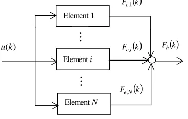
The hysteresis behaviour can be described as a parallel connection (Fig.1) of elementary models [3, 5] with un-known parameters.

Element 1

Element i

Element N )

(k

u Fh

( )

k

( )

k Fe 1,

( )

k F_e,i

[image:1.595.325.511.554.672.2]

( )

k F_e,N

Fig. 1. Model of the hysteresis force based on parallel connection of elementary models

Each elementary model has one common displacement input u

( )

k and one output force Fe,i

( )

k (unmeasurable). The hysteresis force Fh

( )

k corresponds to the sum

Identification of Hysteresis Functions Using

a Multiple Model Approach

Lyudmila Mihaylova

∗

, Vincent Lampaert, Herman Bruyninckx, Jan Swevers

Katholieke Universiteit Leuven, Department of Mechanical Engineering

Celestijnenlaan 300 B, B-3001 Heverlee, Belgium

( )

∑

( )

=

= N

i i e

h k F k

F

1

, . (1)

of the outputs F_e,i

( )

k of the elementary models. Each elementary model has its own state ζ_i

( )

k and is characterized by two parameters: its maximum force Wi (i.e. W_i∈

[

0,F_max

]

) and the spring constant K ._i

i W

i W

−

i K

i u−ζ i

e

F_,

i

∆

i

[image:2.595.58.281.465.626.2]

∆ −

Fig. 2. The characteristic of the elementary model

i

i

K

) (k i

ζ

i

W

) (k u

Fig. 3. Physical interpretation of the elementary model i

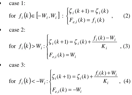
An elementary model relates the relative displacement

( ) ( )

k k

u −ζi to the force Fe,i(k). The relationship is shown in Fig. 2 and can be described by the equations:

• case 1:

for fi

( )

k ∈

[

−Wi,Wi

]

:

  

= = +

) ( ) (

) ( ) 1 (

, k f k

F

k k

i i e

i

i ζ

ζ

, (2)

• case 2:

for f_i

( )

k >W_i:

    

=

− + = +

i i e

i i i i i

W k F

K W k f k k

) (

) ( ) ( ) 1 (

,

ζ ζ

, (3)

• case 3:

for f_i

( )

k <−W_i:

    

− =

+ + = +

i i

e

i i i i i

W k F

K W k f k k

) (

) ( ) ( ) 1 (

,

ζ ζ

, (4)

where f_i

( )

k =K_i

[

u

( ) ( )

k −ζ_i k

]

is the switching para-meter. Each elementary model can be considered as an elasto-slide element consisting of a massless block subject to a Coulomb friction connected to a massless linear spring (See Fig. 3). The parameter W representsi the Coulomb friction and the coefficient K characteri-i zes the spring constant. Another characteristic parameter of the elementary model which can be used is

i

∆ =W /i Ki, i=1,2,...,N, corresponding to the

defor-mation of the spring when the spring force equals the Coulomb friction force. The deformation of the spring is the difference of the input displacement u

( )

k and the position ζ_i

( )

k of the element. When the spring force is larger than the Coulomb friction force, the element begins to slide. Each block of an elementary model can remain in the same position called sticking (case 1), or can undergo a change of the position, called slipping (case 2 and 3). The parallel connection of the different elasto-slide elementary models (Fig.1) form the global static hysteresis model.

On the basis of (2)-(4), the following state-space description can be obtained

x_i

( )

k+1 =F_ix_i

( )

k +G_iu

( )

k +G_η,iη_i

( )

k , (5) y_i

( )

k =C_ix_i

( )

k +D_iu

( ) ( )

k +ξ_i k , (6) where the state x_i

( )

k =ζ_i

( )

k is the position of the i -th element, u

( )

k is the input signal, y_i

( )

k =F_e,i(k) is the output of the element. The respective model parameters are:

• case 1: for f_i

( )

k ∈

[

−W_i,W_i

]

1

=

i

F , Gi =0, Ci =−Ki, Di =Ki; (7)

• case 2: for f_i

( )

k >W_i

( )

i i

i k W /K

x =− , Fi =1,Gi =1, i

i K

C =− ,D_i =0; (8)

• case 3: for f_i

( )

k <−W_i

( )

i i

i k W /K

x = ,

1

=

i

F , G_i =1, C_i =−K_i, D_i =0. (9)

( )

k

i

η and ξ_i

( )

k are process and measurement noises, mutually uncorrelated, Gaussian, zero-mean, with cova-riances Q and i R . i Gη,i allows to change the influence of the process noise η_i, reflecting model and discreti-zation errors due to the replacement of ∆i and K withi grid values from uncertainty domains. There are N2 parameters to identify, namely, W and i K (i i=

N , , 2 ,

1 is the number of the elementary models used). The connected in parallel N elementary models form an augmented single-input single-output model

( )

k Fx

( )

k Gu

( )

k G

( )

k

x 1 ~~ ~ ~_ηη

~ _{+ = + + , (10)}

y

( )

k =C~x

( )

k +D~u

( ) ( )

k +ξ k , (11)

where ~x

( )

k+1 =[ζ₁(k+1), ,ζ_N(k+1)]T, y(k)=Fh(k) N

I

F~= , G~=[G1, ,G_N]T,

T N G G

G~η =[ η,1, , η, ] , ]

, , [ ~

1 KN K

C= − − ,

T N D D

D~=[ 1, , ] , N

I denotes the identity matrix. The parameters K and_i i

III. HYSTERESIS FUNCTION IDENTIFICATION AND

REGIMES DETECTION WITH IMM ESTIMATOR

The MM estimation [6] is based on a grid of the un-known parameters and variables. In the considered prob-lem the unknown parameters are K and the related_i with them variables ∆_i. A set of grid values for ∆_i,

N

i=1,2,..., is formed from physical restrictions, i.e. the maximal ∆_i is determined by the maximal amplitude of the input signal. The uncertainty interval of the spring constants, [K_i,min,K_i,max] can be determined by looking to the minimal and maximal slopes of the measured hysteresis function. Then with each ∆i a grid of spring constants K (i.e. _i K_i,1,K_i,2, ,K_i,q) is formed, covering well the interval [Ki,min,Ki,max]. For each elementary model i a separate IMM estimator is run, with j=1,2,...,q linear Kalman filters (KF)

) ( ) / ( ˆ ) / 1 (

ˆ_, k k F_, x_, k k G_,uk

xij + = ij ij + ij , (12)

) 1 ( ) 1 ( ) / 1 ( ˆ ) 1 / 1 ( ˆ _, , ,

, k+ k+ =x k+ k +K k+ k+

x _ij

j i F j i j

i ν , (13)

) / 1 ( ˆ ) 1 ( ) 1 ( _,

,j k yk yij k k

i + = + − +

ν , (14)

j i T j i j i T j i j i j i j

i k k F P k k F G Q G

P , , , , , ,

, ( +1/ )= ( / ) + η η , (15)

j i T j i j i j i j

i k C P k kC R

S, ( +1)= , , ( +1/ ) , + , , (16)

) 1 ( ) / 1 ( ) 1

( _{, , ,}1

, + = + + − _k S C k k P k

K _{ij i}T_{j ij}

j i

F , (17)

(

)

(

)

( ) ( )

1 1

( )

1 / 1 1 / 1 , , , , , + + + − + = + + k K k S k K k k P k k P j i T F j i j i F j i j i (18)

working in parallel. Each Kalman filter uses the state-space model (5)-(6) with one of its three cases, depen-ding on the switching parameter fi,j

( )

k . The filtered and predicted estimates of x_i,j(k) are xˆi_,j(k+1/k+1) and xˆi_,j(k+1/k) respectively; νi,j(k+1) and Si,j(k+1) are the innovation process and its covariance; KF_i,j(k)

is the Kalman filter gain (note the difference with Ki,j

which is the spring constant); Pi,j(k) is the error

cova-riance; yˆ_i,j

(

k+1/k

)

is the predicted output (according to eq. (6), with parameters of the form (7), (8) or (9), depending on the value of f_i,j(k)). The number of grid values for ∆_i is equal to the number N of elementary models and the dimension of the state vector ~ kx( ). The q grid values for the spring constants determine the number of the KFs.

Using the MM approach [6], the estimated state xˆ_i

( )

k/k of each i -th elementary model can be represented as a fusion of j state estimates xˆ_i,j(k/k)of the KFs , weighted by the mode probabilities µ_i,j

( )

k

( )

∑

( ) ( )

= = q j j i j i

i k k x k k k

x 1 , , / ˆ /

ˆ µ .

For each i -th elementary model an IMM filter is syn-thesized and its mode probabilities are used to compute the averaged elementary model state estimate. Each i -th estimate Kˆ ki( ) can be found as a fusion of values from the preliminary given set, probabilistically weighted by the IMM mode probabilities

( )

∑

= = q j j i j i

i k K k

K 1 , , ) (

ˆ _{µ .}

Based on the grid values for ∆_i and the estimates

) ( ˆ k

Ki , the respective estimated force coefficients

) ( ˆ k

Wi can be computed. The total estimated output (the hysteresis force) is the sum of estimated outputs from the elementary models

( )

_∑

( )

=

= N

i i

h k k y k k

F 1 / ˆ / ˆ _, where

∑

= = q j j i j i

i k k y k k k

y 1 , , ( / ) ( ) ˆ ) / (

ˆ µ .

In the case of multiple elementary models, the innova-tion process νi,j(k+1) of the j -th Kalman filter within the i -th IMM estimator is computed as follows

∑

≠ = + − + − + = + N i l l l j i j

i k yk y k k y k k

, 1 ,

, ( 1) ( 1) ˆ ( 1/ ) ˆ ( 1/ )

ν ,

where the predicted outputs from the elementary models i

l N

l=1, , , ≠ are subtracted from the measured out-put y(k+1). The output from each elementary model is computed as a fusion of the KFs' outputs weighted by the respective IMM mode probabilities.

For each elementary model the different behavior – sticking or slipping can be determined by using the information provided by the probabilities. The probabili-ty whose value is greater than a preset threshold µ_T, i.e.

( )

T j

i j

k maxµ_, >µ

is considered as corresponding to the true regime.

IV. SIMULATION RESULTS

A. Results with one elementary model

In the first simulation the hysteresis function consists of one elementary model (5)-(9) with 1

, 1j =

G_η and a known parameter ∆1= 0.55. A hysteresis function of one

elementary model corresponds to a backlash phenome-non. The parameters to identify are K and ₁ W . A grid₁ of values for K is made, ₁ K1,_grid ={0.1, 0.2, 0.3, 0.4}.

is within the uncertainty interval [0.1,0.4]. The transition probability matrix Pr and the initial mode probability vector µ

( )

0 are

   

 

   

 

=

994 0 002 . 0 002 . 0 002 . 0

002 . 0 994 0 002 . 0 002 . 0

002 . 0 002 . 0 994 0 002 . 0

002 . 0 002 . 0 002 . 0 994 0

. . . .

Pr ,

( )

   

 

   

 

=

4 / 1

4 / 1

4 / 1

4 / 1

0

µ .

The probabilities µ_{1 j,}

( )

0 , j=1,2,3,4, characterizing the possible values of K , are chosen to be equal. The ini-1

tial true state variables are x_1,j

( )

0 =0, whereas the initial estimated states xˆ_{1 j,} (0) are generated as random uniformly distributed numbers within the interval

( )

0,1 . The Kalman filters are run with initial state estimate covariances P_1,j =105 and noise covariances:

(

)

2

,

1 0.001N

Q _j= , R_1,j =

(

0.1µm

)

2, Q_u =

(

0.05µm

)

2. The input signal has been selected of the form [5]

( )



  

       

=sin k sin * k

k u

16 30 2 16

2π π

.

The data are obtained with a sampling interval 002

. 0

=

T s. The results presented are received by ave-raging over 30 Monte Carlo experiments. The real plant force F_h

( )

k , modeled by one element, the estimated plant force Fˆh

( )

k , and the IMM probabilities are given

[image:4.595.369.503.138.256.2]

in Figs. 4-6, respectively. The shape of the estimated hysteresis function is close to the shape of the modeled one as shown in Figs. 4 and 5. The mode probabilities

Fig. 4. Plant force modeled by one elementary model

Fig. 5. Estimated plant force

closest to the true parameter value (Fig. 6). The error

( )

k F

( )

k F

( )

k

e = h − ˆh between the estimated and real force is close to zero (Fig. 7). The estimation accuracy,

Fig. 6. The IMM mode probabilities

[image:4.595.77.248.471.589.2]

Fig. 7. Error between the estimated and real force

Fig. 8. The estimated coefficient Kˆ1

( )

k

Fig. 9. Switching between the three "cases" in the real model for a single run

-1.5 -1 -0.5 0 0.5 1 1.5

-0.2 -0.15 -0.1 -0.05 0 0.05 0.1 0.15 0.2

] [

), (

N k F_h

] [ ),

(k m

u µ

0 0.5 1 1.5 2

0 0.2 0.4 0.6 0.8 1

) (

1 k

µ µ3(k)

) ( 2 k

µ µ4(k)

time, [s]

0 0.5 1 1.5 2

-0.02 0 0.02 0.04 0.06 ] [

), (

N k e

time, [s]

0 0.5 1 1.5 2

0.15 0.2 0.25 0.3 0.35

) ( ˆ

1 k

K

time, [s]

-1.5 -1 -0.5 0 0.5 1 1.5

-0.2 -0.15 -0.1 -0.05 0 0.05 0.1 0.15 0.2

) (

ˆ _k

F_h

] [ ),

(k m

u µ

0 0.5 1 1.5 2

1 1.5 2 2.5 3

[image:4.595.77.246.618.737.2]

[image:5.595.347.506.116.228.2]

characterized by this error with respect to the real force is less than 5 %. The estimated spring constant varies around its true value (Fig. 8). The three cases in the model (5)-(6) are denoted respectively by 1, 2 and 3. Switching between the three cases in the real model is given in Fig.9. The error between real switching and switching observed based on the biggest IMM probability (the third one) are presented in Fig. 10.

Fig. 10. Error between real switching and switching ob-served based on the biggest probability for a single run

B. Results with more elementary models In this experiment the real hysteresis function is simulated with ten elementary models (5)-(9), with

1

,j = i

G_η and

i

∆

={0.05, 0.1, 0.15,0.20, 0.25,0.35,0.55,0.65,0.85, 1},

=

i

K {0.4,0.25,0.25,0.38, 0.10,0.40,0.15,0.12,0.30,0.4}. It means that the augmented model (10)-(11) is of order ten (unknown to the designer). The hysteresis behavior resulting from this augmented model is now approxi-mated with a reduced order augmented model consisting of seven elementary models. Preliminary the uncertainty intervals for the parameters are determined, i.e.

] 1 , 0 (

∈

i

∆ and K_i∈[0.1,0.4].With each elementary mo-del a separate IMM estimator is implemented with the same transition probability matrix, mode probabilities, initial conditions for the state estimates (random, uniformly distributed) and noise covariances as in the first experiment. The grid for ∆_i is : ∆i,grid={0.03, 0.1,

0.2, 0.4, 0.6, 0.8, 1} and for all spring constants: K_i,_grid

={0.1, 0.2, 0.3, 0.4}. Compared to the exact values, three grid values of ∆_i coincide with their exact values, the others are not the same, but are within the un-certainty interval. Also some grid values ofK coincide_i with the exact ones, but the most of them - not. The real hysteresis force F_h

( )

k , its estimate Fˆ_h

( )

k , the error

) (k

e between them and the estimated coefficients

( )

k

Kˆ_i , i=1,...,7 are given in Figs. 11–14. As seen from Figs. 11 and 12, the shapes of the estimated and real hysteresis functions are close. The estimation error is

small (less than 5 %) (Fig.13). The estimated coeffi-cients vary around their true values (Fig.14).

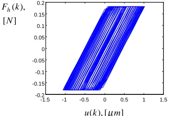
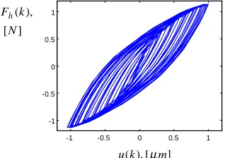
[image:5.595.103.235.191.310.2]

Fig. 11. The real hysteresis force, modeled by 10 ele-mentary models

[image:5.595.340.507.264.382.2]

Fig. 12. The estimated hysteresis force by 7 elementary models

[image:5.595.345.510.419.534.2]

Fig. 13. Error between the estimated and real force

Fig. 14. Estimated coefficients Kˆ ki( )

The examples considered illustrate that through the MM approach the discontinuity (switching) in the state and output models can be overcome.

0 0.5 1 1.5 2

-2 -1.5 -1 -0.5 0 0.5 1 1.5 2

time, [s]

-1 -0.5 0 0.5 1

-1 -0.5 0 0.5 1

] [

), (

N k Fh

] [ ), (k m u µ

-1 -0.5 0 0.5 1

-1 -0.5 0 0.5 1

] [

), ( ˆ

N k F_h

] [ ),

(k m

u µ

0 0.5 1 1.5 2

-0.1 -0.05 0 0.05 0.1 0.15

] [

), (

N k e

time, [s]

0 0.5 1 1.5 2

0.15 0.2 0.25 0.3 0.35 0.4

) ( ˆ k

K_i

[image:5.595.343.509.574.694.2]

V. COMPARISON WITH THE RLSM

Another possible solution for hysteresis function identi-fication is developed in [5] using the recursive least-squares method (RLSM). Results with high estimation accuracy are presented. The results obtained by the IMM estimator have a comparable accuracy of those from the RLSM. The RLSM requires an additional adaptation of the forgetting factor in the presence of changes in the model parameters, whereas the IMM approach possesses an inherent mechanism to reflect quickly the changes. The parallel structure of the model with three different cases and the IMM estimator give the possibility to model and identify hysteresis func-tions, characterized with a hard nonlinearity as swit-ching. The IMM probabilities provide for each ele-mentary model information about sticking and slipping behavior, that information is not available in the RLSM parameter estimates. In comparison with the results received by the RLSM [5], it is not possible to obtain negative values of the estimated parameters due to the fact that the probabilities can only have a positive sign. The IMM implementation does not require considerable computations. In every moment only one of the cases of the elementary model is active. For N parallel elemen-tary models and a grid with q values for K , the numberi of active Kalman filters at each moment is Nq . Advan-tage of the RLSM is that it works almost without initial information, whereas for the IMM the transition probability matrix should be preset. But the transition probabilities are chosen to correspond to the fact that one value of the spring coefficient is the most probable and this simplifies its determination. The crucial point of each MM estimator is the grid construction of the uncertain parameters. The true parameter values have to be within the preset uncertainty intervals.

VI. CONCLUSIONS

This work presents a solution for static hysteresis func-tion identificafunc-tion with a multiple model approach. The hysteresis function is described by a set of elementary models connected in parallel. This parallel structure of the model, in combination with the IMM estimator gives the possibility to reduce the nonlinear identification problem to a linear one. For the parameters (the spring constant and the force coefficient) of each elementary model, grids of possible values are preset taking into account physical restrictions. With each elementary model a separate IMM estimator is synthesized working by linear Kalman filters based on models with different parameters. The final estimate of each parameter represents a fusion of the values from the grid weighted by the IMM mode probabilities. The estimated output of each elementary model is a fusion of the weighted estimates of the Kalman filters by the probabilities, and the total hysteresis force represents the sum of the estimated outputs of all elementary models. A compari-son with the recursive least-squares method is discussed.

Results from simulation experiments with one and more elementary models are presented.

Acknowledgments

H. Bruyninckx is a Postdoctoral Fellow of the Fund for Scientific Research-Flanders (F.W.O) in Belgium. Fi-nancial support by the Belgian Programme on Inter-University Attraction Poles initiated by the Belgian State-Prime Minister's Office-Science Policy Prog-ramme (IUAP). The F.W.O. under grant G.0295.96N, K.U.Leuven's Concerted Research Action GOA/99/04 and grant I-808/98 with the Bulgarian National Science Fund are gratefully acknowledged.

REFERENCES

[1] Barabanov N., and R. Ortega, Necessary and Suffici-ent Condition for Passivity of the LuGre Friction Model, IEEE Trans. on Automatic Contol., Vol.45, No.4, pp.830-832, 2000.

[2] Canudas de Wit, C., H. Olsson, K. Åström and P. Lipchinsky, A New Model for Control of Systems with Friction, IEEE Trans. on Automatic Control, Vol. 40, No.5, pp.419-425, 1995.

[3] Goldfarb, M., and N. Celanovic, A Lumped Parame-ter Electromechanical Model for Describing the Nonli-near Behavior of Piezoelectric Actuators, Trans. of ASME, J. Dynamic Syst., Measurement, and Contr., Vol. 119, pp. 478-485, Sept 1997.

[4] Kuhnen, K. and Janocha H., Adaptive Inverse Control of Piezoelectric Actuators with Hysteresis Operators, Proc. of European Control Conf., 1999. [5] Lampaert, V., and J. Swevers, On-line Identification of Hysteresis Functions with Nonlocal Memory, Proc. of Advanced Intelligent Mechatronics Conference, Como, Italy, 8-11 July, 2001.

[6] Li, X. R. Hybrid Estimation Techniques. Control and Dynamic Systems. (Ed. C.T.Leondes), Vol. 76, pp. 213-287, Academic Press, Inc., 1996.

[7] Mihaylova, L., State Estimation by IMM Filter in the Presence of Structural Uncertainty, Recent Advan-ces in Signal ProAdvan-cessing and Communications, Ed. N. Mastorakis, WSES Press, Greece, 1999, pp.83-88.

[8] Mihaylova, L., Semerdjiev, E., and X.R. Li, Detec-tion and LocalizaDetec-tion of Faults in System Dynamics by IMM Estimator, Proc. of the Second Intern. Conf. on Multisource-Multisensor Information Fusion, 1999, Sunnyvale, California, USA, pp.937-943.

[9] Swevers, J. F. Al-Bender, C. Ganseman, T. Prajogo, An Integrated Friction Model Structure with Improved Presliding Behavior for Accurate Friction Compensa-tion, IEEE Trans. on Automatic Control, Vol.45, No.4, pp.675-686, 2000.