Stochastic Restricted Maximum Likelihood Estimator in Logistic Regression Model

(1)

http://dx.doi.org/10.4236/ojs.2015.57082

Stochastic Restricted Maximum Likelihood

Estimator in Logistic Regression Model

Varathan Nagarajah1,2_{, Pushpakanthie Wijekoon}3

1_{Postgraduate Institute of Science, University of Peradeniya, Peradeniya, Sri Lanka} 2_{Department of Mathematics and Statistics, University of Jaffna, Jaffna, Sri Lanka}

3_{Department of Statistics and Computer Science, University of Peradeniya, Peradeniya, Sri Lanka}

Received 2 November 2015; accepted 27 December 2015; published 30 December 2015

This work is licensed under the Creative Commons Attribution International License (CC BY). http://creativecommons.org/licenses/by/4.0/

Abstract

In the presence of multicollinearity in logistic regression, the variance of the Maximum Likelihood Estimator (MLE) becomes inflated. Şiray et al. (2015) [1] proposed a restricted Liu estimator in lo-gistic regression model with exact linear restrictions. However, there are some situations, where the linear restrictions are stochastic. In this paper, we propose a Stochastic Restricted Maximum Likelihood Estimator (SRMLE) for the logistic regression model with stochastic linear restrictions to overcome this issue. Moreover, a Monte Carlo simulation is conducted for comparing the per-formances of the MLE, Restricted Maximum Likelihood Estimator (RMLE), Ridge Type Logistic Es-timator(LRE), Liu Type Logistic Estimator(LLE), and SRMLE for the logistic regression model by using Scalar Mean Squared Error (SMSE).

Keywords

Logistic Regression, Multicollinearity, Stochastic Restricted Maximum Likelihood Estimator, Scalar Mean Squared Error

1. Introduction

In many fields of study such as medicine and epidemiology, it is very important to predict a binary response riable, or to compute the probability of occurrence of an event, in terms of the values of a set of explanatory va-riables related to it. For example, the probability of suffering a heart attack is computed in terms of the levels of a set of risk factors such as cholesterol and blood pressure. The logistic regression model serves admirably this purpose and is the most used for these cases.

(2)

, 1, ,

i i i

y =π ε+ i=  n (1)

which follows Bernoulli distribution with parameter πi as

( )

exp

, 1 exp

i i

i x

x

β π

β

′ =

′

+ (2)

where xi is the th

i row of X, which is an n×

(

p+1

)

data matrix with p explanatory variables and β is a

(

p+ ×1

)

1 vector of coefficients, εi is independent with mean zero and variance πi

(

1−πi

)

of the response i

y . The maximum likelihood method is the most common estimation technique to estimate the parameter β , and the Maximum Likelihood Estimator (MLE) of β can be obtained as follows:

1 MLE

ˆ _{C X WZ}_{ˆ ,}

β ₌ − _′

(3)

where C=X WX′ˆ ; Z is the column vector with ith element equals logit

( )

ˆ

₍

ˆ

₎

ˆ 1 ˆ

i i

i

i i

y π

π

π π

− +

− and

(

)

ˆ _diag _ˆ ₁ _ˆ

i i

W = _π −π _, which is an unbiased estimate of β . The covariance matrix of βˆMLE is

( )

{



}

1

MLE

ˆ _.

Cov β X W X

−

′

= (4)

As many authors have stated (Hosmer and Lemeshow (1989) [2] and Ryan (1997) [3], among others), the lo-gistic regression model becomes unstable when there exists strong dependence among explanatory variables (multi-collinearity). For example, we suppose that the probability of a person surviving 10 or more extra years is modelled using three predictors Sex, Diastolic blood pressure and Body mass index. Since the response “wheth-er the p“wheth-erson surviving 10 or more extra years” is binary, the logistic regression model is appropriate for this problem. However, it is understood that the predictors Sex, Diastolic blood pressure and Body mass index may have some inter-relationship within each person. In this case, the estimation of the model parameters becomes inaccurate because of the need to invert near-singular information matrices. Consequently, the interpretation of the relationship between the response and each explanatory variable in terms of odds ratio may be erroneous. As a result, the estimates have large variances and large confidence intervals, which produce inefficient estimates.

To overcome the problem of multi-collinearity in the logistic regression, many estimators are proposed alter-natives to the MLE. The most popular way to deal with this problem is called the Ridge Logistic Regression (RLR), which is first proposed by Schaffer et al. (1984) [4]. Later Principal Component Logistic Estimator (PCLE) by Aguilera et al. (2006) [5], the Modified Logistic Ridge Regression Estimator (MLRE) by Nja et al. (2013) [6], Liu Estimator by Mansson et al. (2012) [7], and Liu-type estimator by Inan and Erdogan (2013) [8]

in logistic regression have been proposed.

An alternative technique to resolve the multi-collinearity problem is to consider parameter estimation with priori available linear restrictions on the unknown parameters, which may be exact or stochastic. That is, in some practical situations there exist different sets of prior information from different sources like past expe-rience or long association of the experimenter with the experiment and similar kind of experiments conducted in the past. If the exact linear restrictions are available in addition to logistic regression model, many authors pro-pose different estimators for the respective parameter β . Duffy and Santer (1989) [9] introduce a Restricted Maximum Likelihood Estimator (RMLE) by incorporating the exact linear restriction on the unknown parame-ters. Recently Şiray et al. (2015) [1] proposes a new estimator called Restricted Liu Estimator (RLE) by replac-ing MLE by RMLE in the logistic Liu estimator.

(3)

2. The Proposed Estimator and its Asymptotic Properties

First consider the multiple linear regression model

(

2

)

, ~ 0, ,

y=Xβ ε ε+ N σ I

(5)

where y is an n×1 observable random vector, X is an n×p known design matrix of rank p, β is a p×1

vector of unknown parameters and ε is an n×1 vector of disturbances. The Ordinary Least Square Estimator (OLSE) of β is given by

1 OLSE

ˆ _{S X y}_,

β ₌ − _′

(6) where S=X X′ .

In addition to sample model (5), consider the following linear stochastic restriction on the parameter space

β ;

( )

; 0, 0

r=Rβ ν+ E ν = Covν = Ω > (7) where r is an m×1 stochastic known vector, R is a m×p of full rank m≤p with known elements and ν is an

(

m×1

)

random vector of disturbances with mean 0 and dispersion matrix Ω, and Ω is assumed to be known

(

m m×

)

positive definite matrix. Further it is assumed that ν is stochastically independent of ε , i.e.

( )

0

E εν′ = .

The Restricted Ordinary Least Square Estimator (ROLSE) due to exact prior restriction (i.e. ν =0) in (7) is given by

(

)

1

(

)

1 1

ROLSE OLSE OLSE

ˆ ˆ _{S R RS R} _r _Rˆ

β ₌β ₊ − _′ − _′− ₋ β

(8)

Theil and Goldberger (1961) [10] proposed the mixed regression estimator (ME) for the regression model (2.1) with the stochastic restricted prior information (7)

(

)

1

(

)

1 1

ME OLSE OLSE

ˆ ˆ _{S R} _{RS R} _r _Rˆ

β ₌β ₊ − _′ _{Ω +} − _′ − ₋ β

(9) Suppose that the following linear prior information is given in addition to the general logistic regression mod-el (1)

( )

; 0,

h=Hβ υ+ E υ = Cov υ = Ψ (10)

where h is an

(

q×1

)

stochastic known vector, H is a

(

q×

(

p+1

)

of full rank

(

q≤ +p 1

)

known elements and υ is an

(

q×1

)

random vector of disturbances with mean 0 and dispersion matrix Ψ, and Ψ is assumed to be known

(

q q×

)

positive definite matrix. Further, it is assumed that υ is stochastically independent of

(

)

*

1, 2, , n

ε = ε ε _ ε , i.e. E

( )

ε υ* ′ =0.

Duffy and Santner (1989) [9] proposed the Restricted Maximum Likelihood Estimator (RMLE) for the logis-tic regression model (1) with the exact prior restriction (i.e. υ=0) in (10)

(

)

1

(

)

1 1

RMLE MLE MLE

ˆ ˆ _{C H} _{HC H} _h _H ˆ

β ₌β ₊ − _′ − _′ − ₋ β

(11)

Following RMLE in (11) and the Mixed Estimator (ME) in (9) in the Linear Regression Model, we propose a new estimator which is named as the Stochastic Restricted Maximum Likelihood Estimator (SRMLE) when the linear stochastic restriction (10) is available in addition to the logistic regression model (1).

(

)

1

(

)

1 1

SRMLE MLE MLE

ˆ ˆ _{C H} _{HC H} _h _H ˆ

β ₌β ₊ − _′ _{Ψ +} − _′ − ₋ β

(12)

Asymptotic Properties of SRMLE: The βˆSRMLE is asymptotically unbiased.

(

ˆSRMLE

)

E β =β (13)

(4)

(

)

₁ ₁

(

₁

)

1 ₁ SRMLE

ˆ

Var β =C− −C H− ′ Ψ +HC H− ′− HC− (14)

3. Mean Square Error Matrix Comparisons

To compare different estimators with respect to the same parameter vector β in the regression model, one can use the well known Mean Square Error (MSE) Matrix (MSE) and/or Scalar Mean Square Error (SMSE) criteria.

( ) (

ˆ ˆ

)(

ˆ

)

( ) ( ) ( )

ˆ ˆ ˆ MSE β β, =E_ β β β β− − ′_=D β +B β B′ β

  (15)

where D

( )

βˆ is the dispersion matrix, and B

( ) ( )

βˆ =E βˆ −β denotes the bias vector. The Scalar Mean Square Error (SMSE) of the estimator ˆβ can be defined as

( )

ˆ

( )

ˆ

SMSE β β, =trace MSE_ β β, _ (16) For two given estimators βˆ1 and βˆ2, the estimator βˆ2 is said to be superior to βˆ1 under the MSE

crite-rion if and only if

(

ˆ ˆ1, 2

)

MSE

( )

ˆ1, MSE

( )

ˆ2, 0.

M β β = β β − β β ≥ (17)

The MSE and SMSE of the proposed estimator SRMLE is

(

) (

)

(

)

SRMLE SRMLE SRMLE SRMLE

1

1 1 1 1

ˆ ˆ ˆ ˆ

MSE D B B

C C H HC H HC

β β β β

−

− − − −

′

= +

′ ′

= − Ψ + (18)

(

)

(

)

1

1 1 1 1

SRMLE

ˆ

SMSE β =trace__C− −C H− ′ Ψ +HC H− ′ − HC− __ (19)

(

)

(

) (

)

(

)

MLE SRMLE MLE SRMLE

1

1 1 1

ˆ ˆ ˆ ˆ

Gain in Efficiency MSE MSE D D

C H HC H HC

β β β β

−

− − −

= − = −

′ ′

= Ψ + (20)

Note that the difference given in (20) is non-negative definite. Thus by the MSE criteria it follows that

SRMLE

ˆ

β has smaller Mean square error than βˆMLE.

4. Some Existing Logistic Estimators

To examine the performance of the proposed estimator SRMLE over some existing estimators, the following es-timators are considered.

1) Logistic Ridge Estimator

Schaefer et al. (1984) [4] proposed a ridge estimator for the logistic regression model (1).

(

)

(

)

1 LRE MLE 1 MLE MLE

ˆ ˆ ˆ ˆ

ˆ ˆ

k X WX kI X WX

C kI C Z

β β β β − − ′ ′ = + = + = (21)

where k>0 is the ridge parameter and Zk

(

C kI

)

1C

−

= + . The asymptotic MSE and SMSE of βˆLRE,

( )

(

)(

)

( ) ( ) ( )

(

)(

) (

)

(

)

LRE LRE LRE LRE LRE LRE

1 1

1

1 1

ˆ ˆ ˆ ˆ ˆ ˆ

MSE

k k k k

E D B B

Z C Z Z Z C kI C C kI

β β β β β β β β

β β β β − − δ δ

−  ′ _′ = _ − − _= +   ′ ′ ′ = + − − = + + + (22)

(5)

( )

(

)(

)

(

)

(

)

(

) (

)

(

)

LRE LRE MLE MLE 2 1 2

ˆ ˆ ˆ

SMSE trace

ˆ ˆ

trace

LRE

k k k k

k k E

Z Z Z Z

C Z Z k C kI

β β β β β

β − β

−   ′ =   − −       ′ _′  _′ = _ − − _+ − −    ′  ′ = _ _+ + (23)

2) Logistic Liu Estimator

Following Liu (1993) [11], Urgan and Tez (2008) [12], Mansson et al. (2012) [7] examined the Liu Estimator for logistic regression model, which is defined as

(

) (

1

)

LLE MLE

MLE

ˆ ˆ

ˆ

d

C I C dI Z

β β

β

−

= + +

= (24)

where 0< <d 1 is a parameter and Zd

(

C I

) (

1 C dI

)

−

= + + .

The asymptotic MSE and SMSE of βˆLLE,

( )

(

)(

)

( ) ( ) ( )

(

)(

)

(

) (

)

{

}

{

(

) (

)

}

(

) (

)

(

)

(

)

LLE LLE LLE

LLE LLE LLE 1

1 1 1

2 2

1 1 1

2 2

ˆ ˆ ˆ

MSE

ˆ ˆ ˆ

d d d d

E

D B B

Z C Z Z Z

C I C dI C C I C dI C I C dI I dC C I

β β β β β

β β β

β β β β

δ δ δ δ − − − − − − −  ′ = _ − − _   ′ = + ′ ′ = + − − ′ _′ = + + + + + ′ = + + + + + (25)

where δ2=Zdβ β− .

( )

(

)(

)

(

)

(

)

(

) (

)

(

)

LLE LLE LLE

MLE MLE

2

1 2

ˆ ˆ ˆ

SMSE trace

ˆ ˆ

trace

d d d d

d d E

Z Z Z Z

C Z Z k C kI

β β β β β

β − β

−   ′ = _ _ − − __      ′ _′  _′ = _ − − _+ − −    ′  ′ = _ _+ + (26)

3) Restricted MLE

As we mentioned in Section 2, Duffy and Santner (1989) [9] proposed the Restricted Maximum Likelihood Estimator (RMLE) for the logistic regression model (1) with the exact prior restriction (i.e. υ=0) in (10).

(

)

1

(

)

1 1

RMLE MLE MLE

ˆ ˆ _{C H} _{HC H} _h _H ˆ

β ₌β ₊ − _′ − _′ − ₋ β

(27)

The asymptotic MSE and SMSE of βˆRMLE,

(

ˆRMLE

)

3 3

MSE β = +A δ δ ′ (28)

(

ˆRMLE

)

(

3 3

)

SMSE β =trace A+δ δ (29)

where

(

)

1 1

(

1

)

1 1

RMLE

ˆ

A=D β =C− −C H− ′ HC H− ′ − HC−

and

(

)

1

(

1

)

1

(

)

3 Bias ˆRMLE C H HC H h H ˆMLE

δ ₌ β ₌ − _′ − _′ − ₋ β

(6)

• SRMLE versus LRE

( )

(

)

( ) (

)

{

}

{

( ) ( ) (

) (

)

}

(

)

(

)

{

}

{

(

)

}

(

)

(

)

{

}

(

)

(

)

(

)

{

}

(

)

(

)

1

1 1 ₁ ₁ ₁ ₁

1 1 1

1 1 ₁

1 1 1

1 1

ˆ ˆ

ˆ ˆ ˆ ˆ ˆ ˆ

LRE SRMLE

LRE SRMLE LRE LRE SRMLE SRMLE

MSE MSE

D D B B B B

C kI C C kI C C H HC H HC

C kI C C kI C H H

M N

β β

β β β β β β

δ δ δ δ δ δ − − − − − − − − − − − − − − − − ′ ′ = − + − ′ ′ ′

= + + − − Ψ + +

′ ′

= + + − + Ψ +

′ ′

= + + + − + Ψ

= −

(30)

where M1

(

C kI

) (

1C C kI

)

1 δ δ1 1

− − _′

= + + + and N1

(

C H 1H

)

1

− −

′

= + Ψ . One can obviously say that

(

) (

1

)

1

C+kI − C C+kI − and N1 are positive definite and δ δ1 1′ is non-negative definite matrices. Further by

Theorem 1 (see Appendix 1), it is clear that M1 is positive definite matrix. By Lemma 1 (see Appendix 1), if

(

1

)

max N M1 1 1

λ − _<

, where λmax

(

N M1 11

)

−

is the largest eigen value of N M1 11

−

then M1−N1 is a positive

defi-nite matrix. Based on the above arguments, the following theorem can be stated.

Theorem 4.1. The estimator SRMLE is superior to LRE if and only if λmax

(

N M1 11

)

1

− _<

.

• SRMLE Versus LLE

( )

(

)

( ) (

)

{

}

{

( ) ( ) (

) (

)

}

(

) (

)

(

)

(

)

{

}

{

(

)

}

(

) (

)

(

)

(

)

{

}

(

)

(

) (

)

(

)

(

)

{

}

(

)

(

)

LLE SRMLE

LLE SRMLE LLE LLE SRMLE SRMLE

1

1 ₁ 1 ₁ ₁ ₁ ₁

2 2 1

1 ₁ 1 ₁

2 2 1

1 1 1 1

2 2

ˆ ˆ

MSE

ˆ ˆ ˆ ˆ ˆ ˆ

MSE

D D B B B B

C I C dI I dC C I C C H HC H HC

C I C dI I dC C I C H H

M N

β β

β β β β β β

δ δ δ δ δ δ − − − − − − − − − − − − − − − ₋ − ₋ − ′ ′ = − + − ′ ′ ′

= + + + + − − Ψ + +

′ ′

= + + + + − + Ψ +

′ ′

= + + + + + − + Ψ

= −

(31)

where

{

(

) (

1

)

(

1

)

(

)

1

}

2 2 2

M = C+I − C+dI I+dC− C+I − +δ δ′ and N2

(

C H 1H

)

1

− −

′

= + Ψ . One can obviously

say that

(

) (

1

)

(

1

)

(

)

1

C+I − C+dI I+dC− C+I − and N₂ are positive definite and δ δ₂ ₂′ is non-negative definite matrices. Further by Theorem 1 (see Appendix 1), it is clear that M2 is positive definite matrix. By

Lemma 1 (see Appendix 1), if λmax

(

N M2 21

)

1

− _<

, where λmax

(

N M2 21

)

−

is the the largest eigen value of

1 2 2

N M− then M2−N2 is a positive definite matrix. Based on the above arguments, the following theorem can

be stated.

Theorem 4.2. The estimator SRMLE is superior to LLE if and only if λmax

(

N M2 21

)

1

− _<

.

• SRMLE versus RMLE

(

)

(

)

(

) (

)

{

}

{

(

) (

)

}

(

)

{

}

{

(

)

}

(

)

(

)

{

}

(

)

{

}

RMLE SRMLE

RMLE SRMLE RMLE RMLE SRMLE SRMLE

1 1

1 1 1 1 1 1 1 1

3 3

1 1

1 1 1 1 1 1

3 3 1

1 1 1 1

3 3

ˆ ˆ

MSE

ˆ ˆ ˆ ˆ ˆ ˆ

MSE

D D B B B B

C C H HC H HC C C H HC H HC C H HC H HC C H HC H HC

C H HC H HC C H H

β β

β β β β β β

δ δ δ δ δ δ − − − − − − − − − − − − − − − − − − − − − − − − ′ ′ = − + − ′ ′ ′ ′ ′

= − − − Ψ + +

′ ′ ′ ′ ′

= Ψ + − +

′ ′ ′ ′

= Ψ + + −

{

(

1

)

1 1

}

(

)

3 3

C H− ′− HC− = M −N

(7)

where M3

{

C H1

(

HC H1

)

1HC 1 δ δ3 3

}

−

− _′ − _′ − _′

= Ψ + + and N3

{

C H1

(

HC H1

)

1HC 1

}

−

− _′ − _′ −

= . One can obviously

say that C H−1 ′

(

Ψ +HC H−1 ′

)

−1HC−1 and N3 are positive definite and δ δ3 3′ is non-negative definite

ma-trices. Further by Theorem 1 (see Appendix 1), it is clear that M3 is positive definite matrix. By Lemma 1

(see Appendix 1), if λmax

(

N M3 31

)

1

− _<

, where λmax

(

N M3 31

)

−

is the the largest eigen value of N M3 31

−

then

3 3

M −N is a positive definite matrix. Based on the above arguments, the following theorem can be stated. Theorem 4.3. The estimator SRMLE is superior to RMLE if and only if λmax

(

N M3 31

)

1

− _<

.

Based on the above results one can say that the new estimator SRMLE is superior to the other estimators with respect to the mean squared error matrix sense under certain conditions. To check the superiority of the estima-tors numerically, we then consider a simulation study in the next section.

5. A Simulation Study

A Monte Carlo simulation is done to illustrate the performance of the new estimator SRMLE over the MLE, RMLE, LRE, and LLE by means of Scalar Mean Square Error (SMSE). Following McDonald and Galarneau (1975) [13] the data are generated as follows:

(

)

1 2

2

, 1

1 , 1, 2, , , 1, 2, ,

ij ij i p

x = −ρ z +ρz + i=  n j=  p

(33)

where zij are pseudo- random numbers from standardized normal distribution and

2

ρ represents the correla-tion between any two explanatory variables. Four explanatory variables are generated using (33). We considered four different values of ρ corresponding to 0.70, 0.80, 0.90 and 0.99. Further four different values of n cor-responding to 20, 40, 50, and 100 are considered. The dependent variable yi in (1) is obtained from the Ber-

noulli (πi) distribution where

( )

exp 1 exp i i i x x β π β ′ = ′

+ . The parameter values of

β β

1, 2,,

β

p are chosen so that

2 1

p j j=β

∑

and

β β

1 = 2= =

β

p.

Moreover, for the restriction, we choose

1 1 0 0 1 1 0 0

0 1 1 0 , 2 and 0 1 0

0 0 1 1 1 0 0 1

H h

−

     

     

=_ − _ = −_ _ Ψ =_ _

 ₋     

     

(34)

Further for the ridge parameter k and the Liu parameter d, some selected values are chosen so that 0≤ ≤k 1

and 0≤ ≤d 1.

The experiment is replicated 3000 times by generating new pseudo-random numbers and the estimated SMSE is obtained as

( )

{

( )

}

(

)(

)

(

)(

)

(

) (

)

(

) (

)

(

) (

)

* 3000 =1

ˆ ˆ ˆ ˆ ˆ

SMSE Mean MSE , Mean

ˆ ˆ ˆ ˆ

Mean Mean

1

ˆ ˆ ˆ ˆ

Mean

3000nsim

tr tr E

E tr E tr

β β β β β β β

     ′    = _ _ =    − −                  ′   ′  = _ _ _ − − ___= _ _ _ − − ___                ′  ′ = _ − − _= − −  

∑

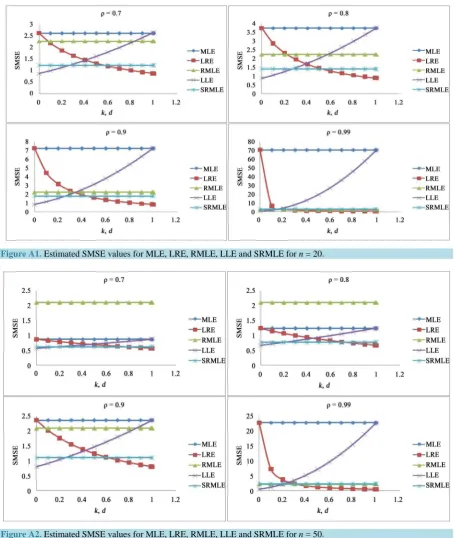
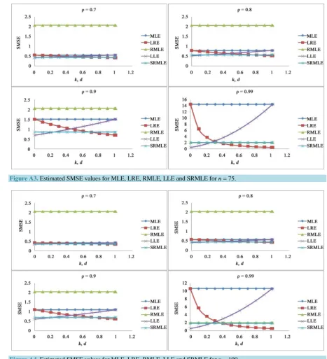
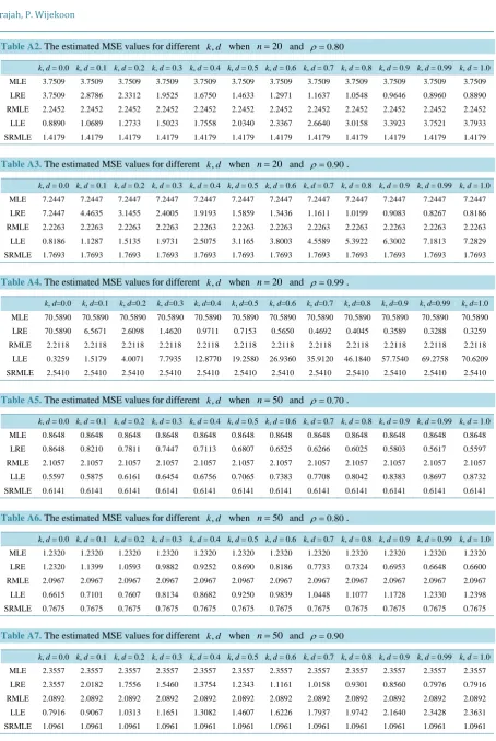
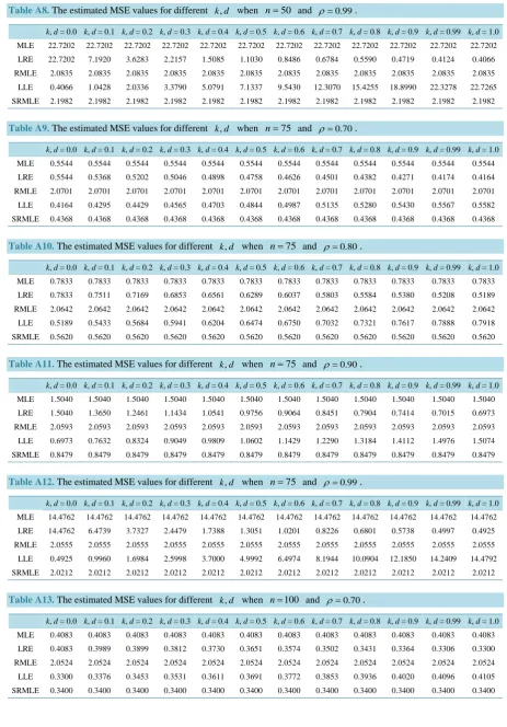
(35)

The simulation results are listed in Tables A1-A16 (Appendix 3) and also displayed in Figures A1-A4

(Appendix 2). From Figures A1-A4, it can be noticed that in general increase in degree of correlation between two explanatory variables ρ inflates the estimated SMSE of all the estimators and increase in sample size n

(8)

SRMLE performs better compared to the estimators LRE, and LLE. From Table A17(Appendix 3), it is clear that when k and d are small LLE is better than other estimators in the MSE sense, and LRE is better when k and

d are large. For moderate k and d values the proposed estimator is good, but this will change with the n and ρ values. Therefore we then analyse the estimators LRE, LLE and SRMLE further by using different k and d val-ues and the results are summarized in Table A18 and Table A19 (Appendix 3). According to these results it is clear that SRMLE is even superior to LRE and LLE for certain values of k and d.

6. Concluding Remarks

In this research, we introduced the Stochastic Restricted Maximum Likelihood Estimator (SRMLE) for logistic regression model when the linear stochastic restriction was available. The performances of the SRMLE over MLE, LRE, RMLE, and LLE in logistic regression model were investigated by performing a Monte Carlo si-mulation study. The research had been done by considering different degree of correlations, different numbers of observations and different values of parameters k, d. It was noted that the SMSE of the MLE was inflated when the multicollinearity was presented and it was severe particularly for small samples. The simulation results showed that the proposed estimator SRMLE had smaller SMSE than the estimator MLE with respect to all the values of n and ρ . Further it was noted that the proposed estimator SRMLE was superior over the estimators LLE and LRE for some k and d values related to different ρ and n.

Acknowledgements

We thank the editor and the referee for their comments and suggestions, and the Postgraduate Institute of Science, University of Peradeniya, Sri Lanka for providing necessary facilities to complete this research.

References

[1] Şiray, G.U., Toker, S. and, Kaçiranlar, S. (2015) On the Restricted Liu Estimator in Logistic Regression Model. Com-munications in Statistics—Simulation and Computation, 44, 217-232. http://dx.doi.org/10.1080/03610918.2013.771742

[2] Hosmer, D.W. and Lemeshow, S. (1989) Applied Logistic Regression. Wiley, New York.

[3] Ryan, T.P. (1997) Modern Regression Methods. Wiley, New York.

[4] Schaefer, R.L., Roi, L.D. and Wolfe, R.A. (1984) A Ridge Logistic Estimator. Communications in Statistics—Theory and Methods, 13, 99-113. http://dx.doi.org/10.1080/03610928408828664

[5] Aguilera, A.M., Escabias, M. and Valderrama, M.J. (2006) Using Principal Components for Estimating Logistic Re-gression with High-Dimensional Multicollinear Data. Computational Statistics & Data Analysis, 50, 1905-1924.

http://dx.doi.org/10.1016/j.csda.2005.03.011

[6] Nja, M.E., Ogoke, U.P. and Nduka, E.C. (2013) The Logistic Regression Model with a Modified Weight Function.

Journal of Statistical and Econometric Method, 2, 161-171.

[7] Mansson, G., Kibria, B.M.G. and Shukur, G. (2012) On Liu Estimators for the Logit Regression Model. The Royal In-stitute of Techonology, Centre of Excellence for Science and Innovation Studies (CESIS), Paper No. 259.

http://dx.doi.org/10.1016/j.econmod.2011.11.015

[8] Inan, D. and Erdogan, B.E. (2013) Liu-Type Logistic Estimator. Communications in Statistics—Simulation and Com-putation, 42, 1578-1586. http://dx.doi.org/10.1080/03610918.2012.667480

[9] Duffy, D.E. and Santner, T.J. (1989) On the Small Sample Prosperities of Norm-Restricted Maximum Likelihood Es-timators for Logistic Regression Models. Communications in Statistics—Theory and Methods, 18, 959-980.

http://dx.doi.org/10.1080/03610928908829944

[10] Theil, H. and Goldberger, A.S. (1961) On Pure and Mixed Estimation in ECONOMICS. International Economic Re-view, 2, 65-77. http://dx.doi.org/10.2307/2525589

[11] Liu, K. (1993) A New Class of Biased Estimate in Linear Regression. Communications in Statistics—Theory and Me-thods, 22, 393-402. http://dx.doi.org/10.1080/03610929308831027

[12] Urgan, N.N. and Tez, M. (2008) Liu Estimator in Logistic Regression When the Data Are Collinear. International Conference on Continuous Optimization and Knowledge-Based Technologies, Linthuania, Selected Papers, Vilnius, 323-327.

(9)

American Statistical Association, 70, 407-416. http://dx.doi.org/10.1080/01621459.1975.10479882

[14] Rao, C.R. and Toutenburg, H. (1995) Linear Models: Least Squares and Alternatives. 2nd Edition, Springer-Verlag, New York, Inc.

(10)

Appendix 1

Theorem 1. Let A: n n× and B: n n× such that A>0 and B≥0. Then A B+ ≥0. (Rao and Toutenburg, 1995) [14].

Lemma 1. Let the two n n× matrices M >0 , N ≥0, then M >N if and only if λmax

(

NM 1

)

1

− _<

. (Rao et al., 2008) [15].

Appendix 2

[image:10.595.86.541.178.717.2]

Figure A1. Estimated SMSE values for MLE, LRE, RMLE, LLE and SRMLE for n = 20.

(11)

[image:11.595.73.541.80.594.2]

[image:11.595.87.543.642.718.2]

Appendix 3

Table A1. The estimated MSE values for different k d, when n=20 and ρ=0.70.

(12)

[image:12.595.86.541.49.727.2]

Table A2. The estimated MSE values for different k d, when n=20 and ρ=0.80

k, d = 0.0 k, d = 0.1 k, d = 0.2 k, d = 0.3 k, d = 0.4 k, d = 0.5 k, d = 0.6 k, d = 0.7 k, d = 0.8 k, d = 0.9 k, d = 0.99 k, d = 1.0 MLE 3.7509 3.7509 3.7509 3.7509 3.7509 3.7509 3.7509 3.7509 3.7509 3.7509 3.7509 3.7509 LRE 3.7509 2.8786 2.3312 1.9525 1.6750 1.4633 1.2971 1.1637 1.0548 0.9646 0.8960 0.8890 RMLE 2.2452 2.2452 2.2452 2.2452 2.2452 2.2452 2.2452 2.2452 2.2452 2.2452 2.2452 2.2452 LLE 0.8890 1.0689 1.2733 1.5023 1.7558 2.0340 2.3367 2.6640 3.0158 3.3923 3.7521 3.7933 SRMLE 1.4179 1.4179 1.4179 1.4179 1.4179 1.4179 1.4179 1.4179 1.4179 1.4179 1.4179 1.4179

k, d=0.0 k, d=0.1 k, d=0.2 k, d=0.3 k, d=0.4 k, d=0.5 k, d=0.6 k, d=0.7 k, d=0.8 k, d=0.9 k, d=0.99 k, d=1.0 MLE 70.5890 70.5890 70.5890 70.5890 70.5890 70.5890 70.5890 70.5890 70.5890 70.5890 70.5890 70.5890 LRE 70.5890 6.5671 2.6098 1.4620 0.9711 0.7153 0.5650 0.4692 0.4045 0.3589 0.3288 0.3259 RMLE 2.2118 2.2118 2.2118 2.2118 2.2118 2.2118 2.2118 2.2118 2.2118 2.2118 2.2118 2.2118 LLE 0.3259 1.5179 4.0071 7.7935 12.8770 19.2580 26.9360 35.9120 46.1840 57.7540 69.2758 70.6209 SRMLE 2.5410 2.5410 2.5410 2.5410 2.5410 2.5410 2.5410 2.5410 2.5410 2.5410 2.5410 2.5410

[image:12.595.86.539.645.719.2]

Table A7. The estimated MSE values for different k d, when n=50 and ρ=0.90

(13)

[image:13.595.79.543.82.747.2]

(14)

[image:14.595.86.537.93.714.2]

[image:14.595.88.540.445.715.2]

Table A17.Summary of the Tables A1-A16.

Best Estimator

n = 20

0.7

ρ = ρ =0.8 ρ =0.9 ρ =0.99

LLE 0.0≤k d, ≤0.2 0.0≤k d, ≤0.2 0.0≤k d, ≤0.2 0.0≤k d, ≤0.1

SRMLE 0.3≤k d, ≤0.5 0.3≤k d, ≤0.5 0.3≤k d, ≤0.4 k d, =0.2

LRE 0.6≤k d, ≤1.0 0.6≤k d, ≤1.0 0.5≤k d, ≤1.0 0.3≤k d, ≤1.0

n = 50

LLE 0.0≤k d, ≤0.1 0.0≤k d, ≤0.2 0.0≤k d, ≤0.2 0.0≤k d, ≤0.2

SRMLE 0.2≤k d, ≤0.7 0.3≤k d, ≤0.7 0.3≤k d, ≤0.6 k d, =0.3

LRE 0.8≤k d, ≤1.0 0.8≤k d, ≤1.0 0.7≤k d, ≤1.0 0.4≤k d, ≤1.0

n = 75

LLE 0.0≤k d, ≤0.1 0.0≤k d, ≤0.1 0.0≤k d, ≤0.2 0.0≤k d, ≤0.2

SRMLE 0.2≤k d, ≤0.8 0.2≤k d, ≤0.7 0.3≤k d, ≤0.6 k d, =0.3

LRE 0.9≤k d, ≤1.0 0.8≤k d, ≤1.0 0.7≤k d, ≤1.0 0.4≤k d, ≤1.0

n = 100

LLE 0.0≤k d, ≤0.1 0.0≤k d, ≤0.1 0.0≤k d, ≤0.1 0.0≤k d, ≤0.2

SRMLE 0.2≤k d, ≤0.8 0.2≤k d, ≤0.8 0.2≤k d, ≤0.7 k d, =0.3

(15)

[image:15.595.81.538.95.352.2]

Table A18.The best estimators and the corresponding k d, values when n=20 and n=50.

n = 20 n = 50

0.7

ρ =

LLE 0.1≤ ≤k 0.6 , 0.1≤ ≤d 0.2 0.1≤ ≤k 0.8 , d=0.1 LRE 0.9≤ ≤k 0.99 , 0.1≤ ≤d 0.2 0.9≤ ≤k 0.99 , d=0.1

0.6≤ ≤k 0.99 , 0.3≤ ≤d 0.99 0.8≤ ≤k 0.99 , 0.2≤ ≤d 0.99 SRMLE 0.1≤ ≤k 0.5 , 0.3≤ ≤d 0.99 0.1≤ ≤k 0.7 , 0.2≤ ≤d 0.99

0.8

ρ =

LLE 0.1≤ ≤k 0.6 , 0.1≤ ≤d 0.2 0.1≤ ≤k 0.8 , 0.1≤ ≤d 0.2 LRE 0.8≤ ≤k 0.99 , 0.1≤ ≤d 0.2 0.9≤ ≤k 0.99 , 0.1≤ ≤d 0.2

0.6≤ ≤k 0.99 , 0.3≤ ≤d 0.99 0.8≤ ≤k 0.99 , 0.3≤ ≤d 0.99

SRMLE 0.1≤ ≤k 0.5 , 0.3≤ ≤d 0.99 0.1≤ ≤k 0.7 , 0.3≤ ≤d 0.99

0.9

ρ =

LLE 0.1≤ ≤k 0.5 , 0.1≤ ≤d 0.2 0.1≤ ≤k 0.6 , 0.1≤ ≤d 0.2 LRE 0.8≤ ≤k 0.99 , 0.1≤ ≤d 0.2 0.1≤ ≤k 0.6 , 0.1≤ ≤d 0.2 0.5≤ ≤k 0.99 , 0.3≤ ≤d 0.99 0.7≤ ≤k 0.99 , 0.3≤ ≤d 0.99

SRMLE 0.1≤ ≤k 0.4 , 0.3≤ ≤d 0.99 0.1≤ ≤k 0.6 , 0.3≤ ≤d 0.99

0.99

ρ =

LLE 0.1≤ ≤k 0.2 , d=0.1 0.1≤ ≤k 0.5 , d=0.1 LRE 0.3≤ ≤k 0.99 , d=0.1 0.6≤ ≤k 0.99 , d=0.1

0.2≤ ≤k 0.99 , 0.2≤ ≤d 0.99 0.4≤ ≤k 0.99 , 0.2≤ ≤d 0.99

[image:15.595.87.542.372.621.2]

SRMLE 0.1≤ ≤k 0.2 , 0.2≤ ≤d 0.99 0.1≤ ≤k 0.3 , 0.2≤ ≤d 0.99

Table A19. The best estimators and the corresponding k d, values when n=75 and n=100.

n = 75 n = 100

0.7

ρ =

LLE 0.1≤ ≤k 0.8 , d=0.1 0.1≤ ≤k 0.8 , d=0.1 LRE 0.9≤ ≤k 0.99 , d=0.1 0.9≤ ≤k 0.99 , 0.1≤ ≤d 0.99

0.8≤ ≤k 0.99 , 0.2≤ ≤d 0.99

SRMLE 0.1≤ ≤k 0.8 , 0.2≤ ≤d 0.99 0.1≤ ≤k 0.8 , 0.2≤ ≤d 0.99

0.8

ρ =

LLE 0.1≤ ≤k 0.8 , d=0.1 0.1≤ ≤k 0.8 , d=0.1 LRE 0.9≤ ≤k 0.99 , d=0.1 0.9≤ ≤k 0.99 , 0.1≤ ≤d 0.99

0.8≤ ≤k 0.99 , 0.2≤ ≤d 0.99

SRMLE 0.1≤ ≤k 0.7 , 0.2≤ ≤d 0.99 0.1≤ ≤k 0.8 , 0.1≤ ≤d 0.99

0.9

ρ =

LLE 0.1≤ ≤k 0.7 , 0.1≤ ≤d 0.2 0.1≤ ≤k 0.8 , d=0.1 LRE 0.9≤ ≤k 0.99 , 0.1≤ ≤d 0.2 0.9≤ ≤k 0.99 , d=0.1

0.7≤ ≤k 0.99 , 0.3≤ ≤d 0.99 0.8≤ ≤k 0.99 , 0.2≤ ≤d 0.99 SRMLE 0.1≤ ≤k 0.6 , 0.3≤ ≤d 0.99 0.1≤ ≤k 0.7 , 0.2≤ ≤d 0.99

0.99

ρ =

LLE 0.1≤ ≤k 0.4 , 0.1≤ ≤d 0.2 0.1≤ ≤k 0.4 , 0.1≤ ≤d 0.2 LRE 0.5≤ ≤k 0.99 , 0.1≤ ≤d 0.2 0.7≤ ≤k 0.99 , 0.1≤ ≤d 0.2