Horror image recognition based on context aware multi instance learning

BIROn - Birkbeck Institutional Research Online

Li, B. and Xiong, W. and Wu, O. and Hu, W. and Maybank, Stephen J.

and Yan, S. (2015) Horror image recognition based on context-aware

multi-instance learning.

IEEE Transactions on Image Processing 24 (12), pp.

5193-5205. ISSN 1057-7149.

Downloaded from:

Usage Guidelines:

Please refer to usage guidelines at or alternatively

Horror Image Recognition Based on Context-Aware

Multi-Instance Learning

Bing Li1, Weihua Xiong1, Ou Wu1, Weiming Hu1*, Stephen Maybank2, Shuicheng Yan3

1

National Laboratory of Pattern Recognition, Institute of Automation, Chinese Academy of Sciences, China

2

School of Computer Science and Information Systems, Birkbeck College, UK

3

Department of ECE, National University of Singapore, Singapore (*Corresponding Author: [email protected])

Abstract Horror content sharing on the Web is a growing phenomenon that can interfere with our daily life and affect the mental health of those involved. As an important form of expression, horror

images have their own characteristics that can evoke extreme emotions. In this paper, we present a

novel context-aware multi-instance learning (CMIL) algorithm for horror image recognition. The

CMIL algorithm identifies horror images and picks out the regions that cause the sensation of horror

in these horror images. It obtains contextual cues among adjacent regions in an image using a random

walk on a contextual graph. Borrowing the strength of the Fuzzy Support Vector Machine (FSVM),

we define a heuristic optimization procedure based on the FSVM to search for the optimal classifier

for the CMIL. To improve the initialization of the CMIL, we propose a novel visual saliency model

based on tensor analysis. The average saliency value of each segmented region is set as its initial

fuzzy membership in the CMIL. The advantage of the tensor-based visual saliency model is that it not

only adaptively selects features, but also dynamically determines fusion weights for saliency value

combination from different feature subspaces. The effectiveness of the proposed CMIL model is

demonstrated by its use in horror image recognition on two large scale image sets collected from the

Internet.

Keywords: horror image recognition, context-aware multi-instance learning, visual saliency

1

Introduction

In the past decades, the explosive growth of Web technologies and resources has allowed us to

conveniently share texts, images, and videos via the Internet from geographically disparate locations.

regularizations allows the distribution of many harmful documents dealing with pornography,

violence, horror, racism, etc. To prevent people, especially children, from accessing the harmful

content on the Internet, many content-based Web filtering systems have been developed [1, 2, 36].

Automatic web filtering is most highly developed for documents with pornographic or violent

content; some filtering systems have matured to a point where they are usefully deployed [1, 2, 36].

In comparison, the automatic recognition and filtering of horror content is still being explored [9, 10,

11]. Many psychological and physiological researches have emphasized the severe effects of horror

images [3, 4, 5]. Field and Lawson [3] point out that exposure to horror increases behavioral

avoidance as well as fears. Ollendick and King [5] also describe an experiment in which 88.8%

children ascribe their fear to negative information acquisition. Many governments have taken

measures to prevent children from seeing horror films, or even passed laws to limit the public

showing of horror films. In the USA, the Motion Picture Association of America (MPAA) categorizes

most horror films as “NC-17” (No Children 17 and Under Admitted) [6, 27]. In 2008, the Chinese

government banned horror films with violent ghosts, monsters, demons, and other inhuman

portrayals [7]. In August 2009, the British Board of Film Censors banned the sale of a Japanese

horror DVD because of its psychological harm to audiences [8]. The severity of the effects of horror

films makes a horror content filtering system a necessity.

1.1 Related Work

Despite the importance of the horror content filtering, most existing work focuses on horror video

recognition. There is, to the best of our knowledge, no specific technique designed for horror image

recognition until now. An intuitive and direct solution is to view “horror” as a specific emotion, and

to apply general affective image classification methods to recognize it.

Normally, human affects can be represented by different emotional words, such as sadness,

excitement, contentment, etc [17, 18]. The basic idea of affective image classification methods is to

investigate the relationship between these high level emotional responses and low level image

features [12]. The affective image classification methods can be divided into two categories: domain

knowledge-based methods and machine learning-based methods [33]. Domain knowledge-based

methods build up hierarchical inference models or rules. Most early methods on image emotion

analysis belong to this category. Kuroda et al. [34] use the color/texture features of segmented image

image. Wang and Yu [13] analyze the emotional meaning embedded in an image through

accumulated knowledge and experience. Methods in the machine learning-based category involve the

training of mapping functions between low-level features and high-level emotional semantics in a

“black box” style. Wang et al. [30] extract image brightness, color temperature, saturation, and

contrast features; and then train an emotion classifier using Support Vector Machines (SVM) [19].

Chen et al. [32] propose to recognize the emotion in an image using a Bayesian classifier based on

color and texture features. Bianchi-Berthouze [14] extracts a set of features from homogeneous

regions in an image and inputs them into neural networks to obtain the emotion information. Fuzzy

neural networks are introduced by Guo and Gao [31] into image emotion recognition. Yanulevskaya

et al. [15] classify images into 8 emotional categories using an SVM classifier with holistic Weibull

and Gabor texture features. Solli and Lenz [16] propose a color-based bag-of-emotions model to

retrieve images associated with particular emotions. Liu et al. [33] present a novel

affective-probabilistic latent semantic analysis model based on feature’s tensor representation for

image emotion classification. Machajdik and Hanbury [17] feed an SVM classifier with a set of

effective features inspired by psychology and art theory for affective image classification. Li et al [18]

recently propose a novel bilayer sparse representation model for affective image classification by

combining global and local features.

Figure 1. Images with different contextual cues evoke completely different emotions. The images are from the International Affective Picture System (IAPS) dataset [54].

Although these methods work well in general affective image classification, their performance

on horror image recognition is very limited. It is primarily because most existing affective image

classification methods try to extract and analyze global features while ignoring the interplay among

the regions in an image. However, our observations show that most horror images, in contrast to

essential parts: at least one horror region that stimulates a strong emotional response and a certain

supporting background. The importance of the context between the two parts is demonstrated by

Figure 1. Images including same man but with different objects in his hand create completely

different emotions due to different contextual cues; the left image is pleasing while the right one is

unsettling. Therefore, an effective classifier for horror image recognition should work on both local

regions and their contextual relationships.

1.2 Our Work

To circumvent the problems of general affective image classification, we apply multi-instance

learning (MIL) [22, 23] to the recognition of horror images. In MIL, an image is viewed as a bag and

the regions within it are instances of the bag. Traditional MIL methods treat the instances

independently and do not model the relations between different regions [22-24]. This paper proposes

a novel context-aware multi-instance learning (CMIL) model for horror image recognition. The

experimental results on two large image sets collected from the Internet show that our algorithm

outperforms the other competing methods. Our algorithm is original in the following ways:

 We propose a novel context-aware multi-instance learning model (CMIL) that classifies a bag by taking into account both individual instances’ labels and their contextual interplay.

 We extend the Fuzzy Support Vector Machine (FSVM) [26] into an effective classifier for the CMIL, referred to as “CMIL-FSVM”, that uses a random walk procedure [41] to model the

context among instances.

 We present a novel tensor-based visual saliency model to integrate emotional cues adaptively. The resulting visual saliency maps of training images can be used to improve the initialization of the

CMIL-FSVM.

 We present a specialized horror image recognition system based on the proposed CMIL model. The system can identify the horror images and the underlying horror regions simultaneously

with a set of discriminative visual and emotional features.

The remainder of this paper is organized as follows: Section 2 gives an overview of our work.

Section 3 introduces the details of horror image recognition based on CMIL. Section 4 presents an

improved initialization of the CMIL-FSVM based on the tensor-based visual saliency model. Section

2

System Overview

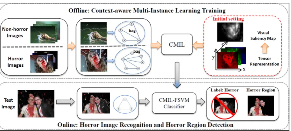
Horror image recognition based on CMIL proceeds in four main stages: bag construction, initial

setting, CMIL classifier training, and horror image recognition. Figure 2 gives an overview of our

system.

Figure 2. Overview of the proposed framework for horror image recognition.

Step 1: Bag construction. We treat each image as a “bag” and all segmented regions in it as “instances”. In each bag, we use an undirected graph to define the contextual relationships between

pairs of regions. The vertices of the graph represent the regions. Two vertices are connected by an

edge if the corresponding regions are adjacent.

Step 2: Initial Setting. In the CMIL-FSVM algorithm, the fuzzy membership of each region in the FSVM for any image is initialized in the training procedure. For the non-horror samples, the

initial fuzzy membership of each region is always fixed to be 1. For the horror images, there are two

possible strategies for determining the initial fuzzy membership: (1) the fuzzy membership of each

region is simply fixed to be a lower value, such as 0.5; or (2) it is gained from the visual saliency map.

In the latter strategy, we compute the visual saliency map of each horror image using the proposed

tensor-based visual saliency model and set the average saliency value of each region as its initial

fuzzy membership.

Step 3: CMIL classifier training. We feed the bag and corresponding initial fuzzy membership values, as well as the label of each training image, into the CMIL and apply the proposed

Step 4: Horror image recognition. For any test image, we segment it into regions and construct its bag. Then, the CMIL classifier is used to predict whether it is a horror image. If it is predicted to

be a horror image, then the classifier further points out the most likely horror region.

3

Horror Image Recognition based on CMIL

In the following, we first describe the context-aware multi-instance learning (CMIL) in detail, and

then discuss its application to horror image recognition.

3.1

Context-Aware Multi-Instance Learning

3.1.1 Formulation of CMIL

Borrowing the formulation of the traditional MIL [22, 23], we add a new matrix term, M_i, into the CMIL definition. The formulation of CMIL is defined as follows: Let χ denote the instance space. Given a data set {(X₁,M₁, ),..., (Y₁ X_i,M_i, ),...(Y_i X_N,M_N,Y_N)} where { _,1,..., _, ,..., _, }

i

i i i j i n

X = x x x ⊆χ

is called a bag, x_{i j,} ∈χ is an instance, and M_i is an adjacency matrix that specifies a contextual graph to model the relations among the instances in the bag X_i. The label of the bag X_i is

={ -1, 1}

i

Y ∈ψ + . The underlying label of any instance is not explicitly given. Different from the traditional MIL [22-24], the underlying label of an instance x_{i j,} in the CMIL is a fuzzy label,

defined as (y_{i j,} ,s_{i j,} )∈θ_i, where y_{i j,} ∈ψ is the class label of x_{i j,} , 0<s_{i j,} ≤1 is the fuzzy membership associated with instance x_{i j,} , and θ_i is the label and fuzzy membership set of the bag

i

X . A hidden contextual score E_{i j,} is defined for each instance x_{i j,} in the bag X_i given the graph

adjacency matrix M_i and fuzzy membership set θ_i. It can be regarded as the tendency of the instance x_{i j,} towards the positive class considering contextual cues among instances in the bag X_i.

The labels of bags in the CMIL model are determined by the contextual scores and can be interpreted

as: If Y_i = +1, then at least one instance x_{i j,} ∈χ has y_{i j,} = +1 and E_{i j,} ≥0.5. If Y_i = −1, then

, 1

i j

(1) Contextual Graph

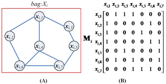
The contextual graph in the CMIL is designed to represent contextual relationship between any

two instances. An example of a contextual graph and its corresponding adjacency matrix M_i are shown in Figure 3. Each vertex of the graph corresponds to an instance in the bag X_i. If there is a

direct contextual link between two instances x_{i j,} and x_{i k,} , the entry in the adjacency matrix,

,

[M_i]_{j k} is set as 1; otherwise it is set as 0. The details of the graph construction for horror images

will be given in Section 3.2.1.

Figure 3. Contextual graph construction: (A) Contextual graph(B) Corresponding adjacency matrix M_i

(2) Contextual Score based on Random Walk

An important step in the CMIL is to compute the hidden contextual score E_{i j,} , for each instance

, i j

x , given the contextual graph. The contextual score E_{i j,} is determined by both the label of x_{i j,}

and the labels of its neighbors. The larger the contextual score Ei j, is, the more possibly positive the

instance x_{i j,} is. To model the contextual scores, we use a random walk on the contextual graph M_i. Random walks on graphs [41] are widely used to define the contextual relevance in many practical

applications, such as Web page ranking [37, 38], and multimedia retrieval [39, 40].

We first transform the fuzzy membership s_{i j,} into a corresponding probabilityvalue p_{i j,} that

represents the conditional probability p y( _{i j,} =1|x_{i j,} ) as

, ,

,

, ,

1,

1 1.

i j i j

i j

i j i j

s if y

p

s if y

= 

Since the probability p_{i j,} includes no contextual information in the bag X_i, it can be viewed as

the independent score of an instance x_{i j,} . We concatenate them together and get an independent

score vector for the bag X_i as [ _,1, _,2,...., _, ]

i T i = pi pi pi n

p . The transition probability matrix

,

[ ]

i = i j k

Q Q in the random walk is defined as [37, 38]

, , , , , [ ] [ ] [ ]

i j k i k i j k

i j m i m m p p =

∑

M , (2)

where [Q_i]_{j k,} is the transition probability from vertex x_{i j,} to vertex x_{i k,} . It actually normalizes the

independent score value of xi k, according to all the adjacency vertices of xi j, .

Given the transition probability matrix Qi, the contextual score

( )

t i j

E + of the instance xi j, at

time t+1 is linearly fused by its neighboring vertices’ contextual scores at time t and its own

independent score p_{i j,} [40, 41] :

( )

( )

, [ ], , (1 ) ,

t t

i j k i k j i k i j

E + =α

∑

where α is the combination weight, [ _{i k j}]_,

( )

k E

∑

contribute to x_{i j,} . If we set [ _,1, _,2,..., _, ]

i T i = Ei Ei Ei n

E , Eq. (3) can be rewritten in the matrix form as

1

(1 )

t t

i i i i

+ _{= + −}

E αQ E α P. (4)

Eq. (4) defines a recursive updating of Et_i. It can be shown that the limit _i lim t_i

t−>∞

=

E E exists [41]. On taking the limit t− > ∞ in (4), it follows that

1

(1 ) ,

(1 )( ) .

i i i i

i i i

which reduces to

α α

α α −

= + −

= − −

E Q E P

E I Q P (5)

Given the contextual score E_{i j,} of each instance x_{i j,} , the label of each bag in the CMIL can be

described in the form of a constraint by

( )

(

)

1maxi 0.5 0

i i j

j n

Y E

≤ ≤

× − ≥ . (6)

3.1.2 CMIL Classifier Optimization via Fuzzy SVM

labels of the instances are always binary. Lin et al. [26] propose the fuzzy SVM (FSVM) in which

each input training sample has a fuzzy class membership. In this paper, we propose an extended

FSVM, named as CMIL-FSVM, in which the contextual score is added as another constraint.

(1) Maximum Pattern Margin via FSVM

The basic idea of CMIL-FSVM is to learn a fuzzy classifier in instances space that can predict

the label and fuzzy membership of each instance in a bag and then determine the bag’s label from

these predictions. Let the classification hyperplane in the instance space be f x( _{i j,} )=wTx_{i j,} +b with the parameter ( , )w b [24]. The optimization objective function of the proposed CMIL-FSVM is

obtained by combining the contextual score constraint [26] and the objective function of the FSVM

as

( )

(

)

subject to ( ) 1 , 0

max 0.5 0

i

i n

i j i j b

i j T

i j i j i j i j

i i j

j n

C s

y x b

Y E ξ ξ ξ = ≤ ≤ + + ≥ − ≥ × − ≥

∑∑

where C is a constant and can be regarded as a regularization parameter. If si j, in Eq. (7) is small,

the effect of the parameter ξ_{i j,} and the corresponding instance x_{i j,} is of less importance to the classification hyperplane.

(2) Optimization Heuristics

The big difficulty to solve Eq. (7) is that, different from the standard classification of the FSVM

in which the labels y_{i j,} and fuzzy membership s_{i j,} are explicitly predefined in the training

procedure, these two terms are not explicitly given out in the CMIL. Inspired by the optimization

procedure of the mi-SVM [24], we present a heuristic procedure to minimize the objective function

defined in Eq. (7). The optimization procedure includes two major steps: fuzzy classification and

label update.

Step 1: Fuzzy Classification. Given the hidden label y_{i j,} and fuzzy membership s_{i j,} of each

instance, the optimization of Eq. (7) is reduced to a quadratic programming problem that can be

Step 2: Label Update. Once the classification hyperplane has been learnt through FSVM, the

hidden label y_{i j,} and fuzzy membership s_{i j,} of each instance will be updated based on the

hyperplane using Eq.(8).

,

, ,

, | ( )|

sgn( ( )),

1 , 1+ i j

i j i j

i j f x

y f x

s e− =    ₌  (8)

Algorithm 1. Pseudo-code for the CMIL-FSVM optimization heuristics.

Training Procedure

INPUT: All the training bags with corresponding labels as

1 1 1

{(X ,M, ),..., (Y X_i,M_i, ),...(Y_i X_N,M_N,Y_N)}. Initialize

, , for ,

i j i i j i

y =Y x ∈X ;

, 1, for , and =-1; , 0.5, for , and =+1

i j i j i i i j i j i i

s = x ∈X Y s = x ∈X Y , ∆ =s 0.1.

REPEAT

Compute the classification hyperplane f x( i j_, ) via the FSVM using all the instances.

Compute outputs

, ,

( ) T

i j i j

f x =w x +b for all x_{i j,} in positive bags. Compute y_{i j,} and s_{i j,} for all x_{i j,} in positive bags using Eq. (8). Set k =0;

For (every positive bag X_i)

Compute

,

i j

E for each instance x_{i j,} in X_i based on Eq. (5). Compute

( )

, 1

* arg max

i i j j n j E ≤ ≤ = If (

, * 0.5

i j

E < )

Set si j_{, *}=min 1,

(

)

Set k = +k 1. END

END

WHILE (k ==0 or maximal iteration number is arrived)

OUTPUT(w,b)

Test Procedure

INPUT: A test bag t

X and corresponding contextual graphMt.

Compute outputs

, ,

( ) T

t j t j

f x =w x +b for all instancesx_{t j,} in t

X .

Compute y_{t j,} and s_{t j,} for all instances x_{t j,} in

t

X .

Compute

,

t j

E for each instance in

t

X based on Eq. (5). Compute

( )

, 1

* arg max t t j j n j E ≤ ≤ = IF (

, * 0.5 t j

E ≥ )

set ₁

t

Y =

ELSE set ₁

t

Y = −

END

OUTPUT(

t

where the sigmoid function is widely used to obtain an output from the SVM in the form of

probabilities.

After obtaining the classifier during the learning procedure, we can compute the label y_{t j,} and

membership s_{t j,} of each instance x_{t j,} in the test bag

t

X using ( , ) ,

T

t j t j

f x =w x +b and Eq. (8). And

the label of

t

X can be determined by the labels and memberships of all the instances in X_t. The

implementation details of the CMIL-FSVM are shown in Algorithm 1.

It is worth noting that, during the initialization stage, we pair positive labels of those instances in

positive bags with lower fuzzy memberships (s_{i j,} =0.5), and negative labels of those instances in

negative bags with higher fuzzy memberships (s_{i j,} =1) so as to make sure that all initial contextual

scores of negative bags are less than 0.5. Then, we iteratively adjust the hyperplane by improving the

fuzzy memberships of positive instances to ensure that the positive bags satisfy the constraints in Eq.

(7).

3.1.3 Differences from Other MIL Methods

Many MIL methods have been proposed in the literatures, in which mi-SVM and MI-SVM [24] are

widely used. Different from the CMIL that considers contextual cues among instances, these two

methods treat all instances from a bag as independently and identically distributed (i.i.d.). The

methods that are closer in spirit to our CMIL are miGraph and MIGraph proposed by Zhou et al. [25].

The main difference lies in the definition of the relationship between instances. The miGraph and

MIGraph algorithms [25] are essentially graph pattern classifiers. They only consider the global

graph structures of a bag and predefine any two instances’ relationship based on a -graph that uses

the Euclidean distance in a feature space; whereas our CMIL considers contextual cues among

instances using a random walk on a spatial adjacency graph. The relationship between any pairs of

instances can be dynamically learnt from the training data.

3.2

Horror Image Recognition based on CMIL

In this section, we apply the proposed CMIL model to horror image recognition using some effective

features.

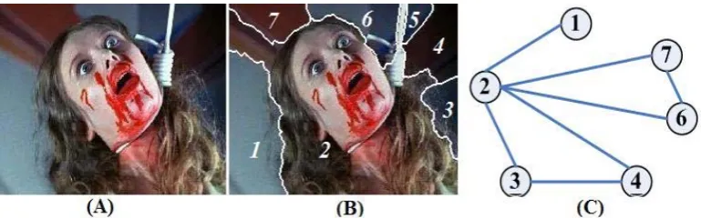
The first step in the horror image recognition based on CMIL is to construct instances, bags and

contextual graphs. The intuitive idea is to treat an image I_i as a bag and segmented regions

,1 ,2 ,

{ , ,..., }

i

i i i n

I I I of the image I_i as instances. Among diverse image segmentation algorithms, the

JSEG algorithm [28] is adopted because of its flexibility. After segmentation, we discard the regions

whose areas are smaller than 1/40 of the image. Figure 4 gives an example of image segmentation by

the JSEG.

The next step is to construct the graph adjacency matrix M using the segmented regions in an image. The vertices of the graph represent the image regions and an edge with weight of 1 is defined

between any two adjacent regions. An example of a bag and the corresponding graph is shown in

Figure 4.

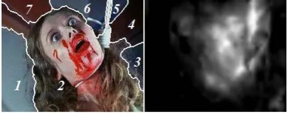
Figure 4. Bag construction: (A) Original image. (B) Segmentation result. (C) Contextual graph. The 5th region is discarded because it is too small.

3.2.2 Feature Extraction

For each region, three types of features, namely color, color emotion, and texture, are extracted,

because they are validated by many affective image classification methods [15, 16, 17].

Color Feature. Colors are often used by artists to induce emotional effects. Here we consider image color information in the CIELAB space because it describes color perception more accurately

than RGB space [13]. Two feature sets are defined as [ ,1 2, 3] [ , , ] k k k

k k k

f f f = L a b and

4 5 6

[ ,fk fk,fk] [= Lk−L a, k−a b, k−b]. The former set is the average of all the pixels’ CIELAB values in the

th

k

region, and the latter set is defined as the difference between averaged pixel value in the th

k region

and that of the whole image.

emotion space with axes representing color activity (CA), color weight (CW), and color heat (CH).

The values of CA, CW and CH are calculated as follows:

1/ 2 2 *

* 2 * 2

* *

* 1.07 *

17

2.1 0.06 ( 50) ( 3) ,

1.4

1.8 0.04(100 ) 0.45 cos( 100 ),

0.5 0.02( ) cos( 50 ),

o

o

b

CA L a

CW L h

CH C h

 _{ − }  = − +  − + − +_{ }        = − + − + − = − + − (9)

where ( ,L a b* *, *)and ( ,L C h* *, *) are the corresponding color values in the CIELAB and CIELCH color spaces for a given RGB color. The average color emotion of the pixels in each region yields a

feature vector [f₇k, f₈k,f₉k] [= CA CW CH_k, _k, _k], and the difference between it and the whole image yields a second feature vector [f₁₀k,f₁₁k,f₁₂k] [= CA_k−CA CW, _k−CW CH, _k−CH].

Texture Feature. Geusebroek et al. [43] describe a stochastic texture perception. They show that the distribution of edge responses can be modeled by a Weibull distributionwb z( )as

1

( )

z

z

wb z e

γ γ β γ β β −   −      =  

  , (10)

where z is the edge responses in a single color channel to the Gaussian derivative filter, β >0 is the scale parameter of the distribution and γ >0 is the shape parameter. The parameters of the Weibull distribution completely characterize the spatial structure of the texture [43] and widely used

in for texture description [14]. The contrast in an image is represented by β, and the grain size is given by γ . Thus, the β and γ values for the x-edges and y-edges in the RGB color channels for each region yield a 12 dimensional feature vector, as [ 13, 14 15, 16] [ , , , ]

k k k k k k k k

xR xR yR yR

f f ，f f = γ β γ β ,

17 18 19 20

[ k, k k, k] [ k , k , k , k ]

xG xG yG yG

f f ，f f = γ β γ β , and [ ₂₁k, ₂₂k ₂₃k, ₂₄k] [ k , k , k , k ]

xB xB yB yB

f f ，f f = γ β γ β . In addition, the texture differences between the current region and the whole image are also used as texture features:

25 26 27 28

[ ,fk fk，fk,fk] [= γ γ β β γ γ β β_xRk − _xR, _xRk − _xR, _yRk − _yR, _yRk − _yR] , [ ,f₂₉k f₃₀k，f f₃₁k, ₃₂k] [= γ_xGk −γ β_xG, _xGk −β γ_xG, _yGk −γ β_yG, _yGk −β_yG] , and

33 34 35 36

[fk,fk，fk,fk] [= γk_xB−γ β_xB, _xBk −β γ_xB, _yBk −γ β_yB, _yBk −β_yB].The concatenation of all these features yields a feature vector in R36 for each region.

Given the contextual graph of an image and feature vector of each region in it, we can construct a bag

for each image in the CMIL. Now the bag X_i represents the whole image I_i; the instance

36 , [ 1 , 2 ,..., 36]

j j j

i j

x = f f f ∈R is the feature vector of the jth region in the image I_i; M_i is the spatial contextual graph matrix of the image; and the label Y_i for each image is set to 1 if it is a

horror image, and otherwise is set to -1. All the bags of the training images and their corresponding

labels are input to the CMIL to learn a classifier using the CMIL-FSVM algorithm. Given a test

image, the extracted feature vector of each region and the contextual graph of the image are obtained

in the form of a bag. Then, the bag is fed into the CMIL classifier to identify whether it is a horror

image. Furthermore, if the test image is judged as a horror image, we consider the region with the

highest contextual score to be a horror region in the image.

4

Improved CMIL-FSVM by Visual Saliency Map

In Algorithm 1, the memberships of all the instances in the positive bags are simply set to be 0.5

(s_{i j,} =0.5). This initialization may mislead the classifier, because there often exist instances with

negative labels or much lower positive memberships in positive bags, such as the background of a

horror image. If the CMIL-FSVM is initialized with weak labels and corresponding membership

values based on some prior knowledge, the convergence of the classification optimization algorithm

may be faster, and a more accurate classifier may be obtained.

Because a horror image always contains one or more popped-out region(s) that is (are) very

different from the background in their visual or emotional stimulus. The detection and separation of

these salient regions can provide very valuable initialization information to the CMIL-FSVM. In this

paper, we propose a simple and effective visual saliency model based on tensor reconstruction, and

then discuss how to initialize the CMIL-FSVM using visual saliency maps.

4.1

Emotional Attention Mechanism

Much recent psychological research indicates that emotion is of another fundamental importance in

the human vision system and produces specific contributions to selective attention [20]. Vuilleumier

[21] argues that the amygdala plays a crucial role in providing both direct and indirect signals on

effects implement specialized mechanisms of “emotional attention” that may supplement visual

attention.

In the past decades, many visual saliency computation models [46-52] have been proposed.

Most of them follow Koch’s bottom-up saliency map framework [44, 45] that extracts low level

visual features and combines the visual saliency values in different feature subspaces to produce the

final saliency map [46-52]. Therefore, they have to address two essential questions: (1) find those

features with good discriminating power; and (2) determine each feature’s weight in combination.

Although these elaborate methods achieve good performance, they have the following limitations:

(1) Most existing visual saliency methods predefine several low level features, such as gray intensity,

color channel and local shape orientation, and apply them to all pixels of any input image. These

widely-used features may be effective for general visual saliency models; but there is no evidence to

show that they are effective for modeling the emotional attention. (2) Most existing methods treat

color and texture features separately in visual saliency computation, but research has shown that

using color and texture in combination (i.e. color texture) results in better discrimination [55, 56]. (3)

Some existing methods fuse saliency maps obtained from different feature subspaces. They predefine

a combination weight for the saliency map from each feature subspace. The predefined weights may

yield good performance for some images or certain parts of an image; but they cannot always work

for all images or for all parts of an image containing different types of scene.

To avoid these limitations, we propose a novel visual saliency map model based on tensor

reconstruction that can combine several emotion cues dynamically. In the proposed model, we

represent an image in the color emotion space [42] and organize it as a color emotion tensor structure.

The first few basis elements in the tensor decompositions of neighboring blocks for each pixel are

chosen as features for saliency computation, since they can reveal the most significant information

inherent in the surrounding environment. The reconstruction residual error of the pixel’s feature

based on these basis elements, which shows whether the pixel includes the similar related features to

its neighbors, is used as the visual saliency value. The hypothesis behind the proposed tensor-based

saliency map model is that if a pixel is salient, its appearance (color, texture, etc.) and tensor structure

will be very different from its neighbors’, so the tensor reconstruction residual using its neighbors

will be large. Otherwise, the tensor structure of the pixel is similar to its neighbors’ and the tensor

reconstruction residual will be small.

the following advantages:

 The tensor structure in color emotion space not only represents image’s color values into a unit, rather than 3 separate channels, but also takes into account the spatial interaction within each

channel as well as the interaction between different channels.

 We need not explicitly extract features for each pixel. Features used for each pixel’s saliency computation are adaptively determined and selected by tensor decomposition.

 The combinational coefficient for each selected feature are not predefined, instead they are dynamically gained from tensor reconstruction.

4.2

Visual Saliency Map Based on Tensor Reconstruction

4.2.1 Tensor Representation

Since the color emotion space is shown to contain more high-level emotional cues than other

color spaces [42], we first represent an image in the color emotion space as in Eq. (9). Then, we

divide the image into blocks with size of w w× pixels and use a 3-order tensor to represent color

values in color emotion channels of each block as w w c

R × ×

∈

B , where w is the row and column sizes of each block, and c=3 is the dimension of the color emotion space. For any pixel with its

location q, the block centered on it is called the “Center Block” (CB). The adjacent blocks with

overlapped w/ 2 pixels yield 16 “Neighboring Blocks” (NB). The CB and NB are 3-order tensors.

All neighboring blocks are further assembled into a 4-order tensor, M∈Rb w w c× × × ₍b=16_{). An}

example is shown in Figure 5.

Figure 5. The center block (CB) of pixel q has 16 overlapped neighboring blocks with w/ 2 overlapping pixels: NB NB₁, ₂,...NB₁₆. Each block is in size of w w× pixels.

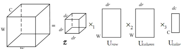
4.2.2 Saliency Map from Tensor Reconstruction

1 block 2 row 3 column 4 color

= × U × U × U × U

M Z , (11)

where × × ×₁, ₂, ₃ and ×₄ are the n-mode product operations of the tensor Z and matrices ,

row column

U U and U_color [53]. Here, the core tensor Z reflects the interactions among 4 subspaces: the matrix U_block spans the subspace of block parameter; the matrix Urowspans the subspace of each

block row’s parameter, includes correlation between any two rows along all blocks, and represents

different texture basis along vertical direction. Similarly, the matrix Ucolumnspans the subspace of

each block column’s parameter, includes correlation between any two columns along all blocks, and

represents different texture basis along horizontal direction. The matrix U_color spans the subspace of color emotion parameter and each eigenvector represents one kind of linear transformation of color

emotion values.

Figure 6. An example of a 4-order Tucker decomposition viewed from 1st Block.

Since U_block only represents the correlation among all neighboring blocks, the decomposition output along this order is not considered in the following analysis. So we keep its dimension to be

16 16× . For the remaining three orders, we take first dr eigenvectors of U_row and U_column to form the basis matrices Udr_row and Udr_column that contain the most important texture energy along

vertical and horizontal directions respectively. We also take the first dc most important linear

transformations of the U_color eigenvectors Udc_color to emphasize color emotion feature variations. An example of this tensor decomposition is given in Figure 6.

During projection and reconstruction, we represent the center block at location q as a 3-order

tensor T ∈Rw w c× × , then project it using Udrrow , dr column

U and Udccolor , the projected tensor is

dr dr dc

R × ×

∈

( )

(

) (

)

1 2 _column 3 _color

T T

T

dr dr dc

row

= × U × U × U

P T . (12)

Then, we get the reconstruction tensor T R of the center block tensor T by multiplying the

projected P with the basis matrices of dr row

U , dr column

U and dc color

U , as

( )

( ) ( )

( )

(

)

(

( )

)

(

( )

)

1 2 3

1 2 3 1 2 3

1 2 3

column color

column color column color

column column color color

R dr dr dc

row

T T

T

dr dr dc dr dr dc

row row

T T

T

dr dr dr dr dc dc

row row

= × × ×

= × × × × × ×

= × × ×

U U U

U U U U U U

U U U U U U

T P

T T

. ₍₁₃₎

After reconstruction, the residual error r q( ) at pixel q is computed as

(

)

, , , , 1 1 1

( )

w w c

R i j k i j k i j k

r

= = =

=

∑∑∑

q T T . (14)

The result r q( ) is used as the saliency value of the processed pixel. In this way, we approximate the

center block’s color emotion and texture pattern by the linear sum of the learned patterns of

neighbors through tensor reconstruction. Obviously, if the central block has similar features with its

neighbors in terms of color emotion and local textures, the principal tensor components gained from

neighboring blocks may be similar to those gained from the center block so that the reconstruction

error is small, otherwise the reconstruction error is higher and the pixel has a large saliency value.

4.2.3 Pyramid Saliency Map Calculation

The pyramid architecture, which is widely used in visual saliency methods, offers a framework

for image saliency map calculation with increased resolution quality [52]. We use a pyramid with L

different levels, denoted as 1 2

, ,..., L

I I I , for the saliency map calculation, where 1

I is the original

image and IL is the lowest resolution image. The value of L is determined to be sure that the

image’s width and height of IL _{are not less than 64 pixels. The normalized saliency map at each}

level is then resized to match the size of the original image. The values of all the saliency maps at

different levels are averaged to gain the final saliency map:

1 1 ˆ ( ) ( ) L l l SM r L = =

∑

q q , (15)

where SM( ) [0,1]q ∈ is the final saliency value of pixel q, ˆ ( )r q_l is the normalized saliency value

4.3

Initialize of the CMIL with Weak Labels Based on Visual Saliency Map

Using the proposed tensor-based visual saliency map model, we obtain a normalized visual saliency

map of each horror image in the training set. As shown in Figure 7, the image regions with high

saliency values in a horror image indicate high emotional stimulus. For each positive training image

(bag) X_i, we compute its visual saliency map SM_i. The average saliency values of all the

segmented region (instance) are also computed as _,1, _,2,..., _,

i

i i i n

SM SM SM . The initial fuzzy

membership s_{i j,} for the instance x_{i j,} in the bag X_i is set as: s_{i j,} =SM_{i j,} , rather than the value of

0.5 used in Algorithm 1.

Figure 7. A horror image with the associated visual saliency map.

5

Experiments

To evaluate the performance of the proposed CMIL for horror image recognition, we compared it

with other prevailing affective image classification methods as well as some MIL methods on two

large scale image sets.

5.1

Data Set and Error Measurement

5.1.1 Data Set

Due to a lack of publicly available image sets for horror image recognition, we collected two horror

image sets from the Internet. One set includes 1000 horror and non-horror images (referred to as

1000 Horror Image Set). The other one includes 10,000 horror and non-horror images (referred to as

10000 Horror Image Set).

(1) 1000 Horror Image Set

This horror image set includes 500 horror images and 500 non-horror images. To collect the

search engines (google.com, bing.com, baidu.com) with related query words, such as “horror”, “fear”,

“bloody”, and corresponding Chinese words. We invited 7 students in our laboratory to label each

image as one of three categories: Non-horror, A little horror, and Horror. Then, we selected 500

images, each of which was labeled as “Horror” by at least 4 users. We also selected 500 non-horror

images with different scenes, objects or emotions. These non-horror images include 50 indoor images,

50 outdoor images, 50 human images, 50 animal images, 50 plant images, and 250 images with

emotional associations (adorable, amusing, boring, exciting, irritating, pleasing, and surprising). The

non-horror images were downloaded from the famous image retrieval system ALIPR, with website

(http://alipr.com/) using a range of different emotional query words.

In addition, in order to evaluate the performance of the proposed visual saliency map

computation model, these 7 students were also required to draw a bounding box around the most

salient horror region for each horror image in this set (according to their understanding). The

bounding boxes in each image were averaged to get the ground truth of the visual saliency map,

( )

EM q [48]:

( ) { | [0,1]}

EM q = m_q m_q∈ , where

1

1 U i

i

m a

U =

=

∑

q q (16)

where U =7 is the number of bounding boxes and i {0,1}

a_q∈ is a binary label to indicate whether

or not the pixel q is inside the bounding box given by the ith student.

(2) 10000 Horror Image Set

The second image set includes 10,000 images, in which there are 5000 horror images and 5000

non-horror images. More than 8,000 candidate horror images were downloaded from a horror image

sharing group in a famous image sharing website (flickr.com). The sharing group advises that the

users who upload non-horror subject matter will be pulled out. As a result, all the images from this

group are horrible. Using the same selection procedure as that in creating 1000 image set, we

obtained 5000 horror images after removing duplicates. We also selected 5000 non-horror images

from the COREL database [35] which contains a large number of various scenes and is widely used

for image understanding research.

5.1.2 Error Measurement

For horror image recognition, given the ground truth of a horror image set, referred as HS, and the

measure defined in Eq. (17) were used to evaluate the recognition performance:

1

2

, , .

HS ES HS ES prec rec

pre rec F

ES HS prec rec

× ×

= = =

+

 

(17)

5.2

Horror Image Recognition Based on CMIL without Visual Saliency

In this section, we evaluated the performance of the CMIL in terms of horror image recognition

without the initialization using the visual saliency map, as shown in Algorithm 1.

We compared the CMIL with some general affective image classification methods: the

emotional valence categorization (EVC) algorithm [15], the color based bag-of-emotions (BoE)

model [16], the affective-pLSA based method (APLSA) [33] and the bilayer sparse

representation-based method (BSR) [18]. Although these methods are not specially designed for

horror image recognition, we still used them to classify images as: horror and non-horror. In addition,

the leading MIL algorithms, mi-SVM, MI-SVM [24], miGraph, and MIGraph [25], were also applied

to horror image recognition for comparison. To fairly compare all these MIL methods, the bag

construction and instances’ features in MIL methods are the same as those used in our CMIL.

Moreover, the Radial Basis Function (RBF) was adopted as kernel functions in the CMIL, mi-SVM,

MI-SVM, miGraph, and MIGrpah. The parameter α in Eq. (4) of the CMIL-FSVM was selected from {0.1, 0.3, 0.5, 0.7, 0.9}. The optimal parameters for each algorithm were determined through the

3-cross-validation on the training set in each experiment.

5.2.1 Results on 1000 Horror Image Set

The first experiment is on the 1000 horror image set. For each method, we repeated the 3-fold cross

validation 10 times and used the average performance of the 10 repeats as the final result.

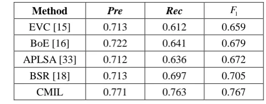
(1) CMIL vs Affective Image Classification Methods

The performance comparisons between the CMIL and other affective image classification methods

are shown in Table 1. The experiment results demonstrate that the CMIL outperforms the completing

methods. The EVC, BoE and APLSA only use global features for affective image classification. The

BSR achieves slightly better performance than the other three affective classification methods due to

the fact that the BSR method combines local and global features for classification. However, the BSR

is essentially a global method in which it does not consider the contextual cues among regions. These

Table 1. Performance comparison with affective image classficiation methods on the 1000 horror image set.

Method Pre Rec F1

EVC [15] 0.713 0.612 0.659

BoE [16] 0.722 0.641 0.679

APLSA [33] 0.712 0.636 0.672

BSR [18] 0.713 0.697 0.705

CMIL 0.771 0.763 0.767

(2) CMIL vs MIL

We compared the proposed CMIL with 4 leading MIL methods, mi-SVM, MI-SVM [24], miGraph,

and MIGraph [25], in terms of horror image recognition on the 1000 horror image set. The mi-SVM

and MI-SVM can be viewed as local methods because they work on image regions. The miGraph,

MIGraph and CMIL are regarded as contextual methods because they take into account the

contextual cues among regions. The experimental results for these methods are listed in Table 2.

Table 2. Performance comparison with other MIL methods on the 1000 horror image set.

Method Pre Rec F1

mi-SVM [24] 0.712 0.726 0.719

MI-SVM [24] 0.693 0.707 0.700

miGraph [25] 0.725 0.732 0.728

MIGraph [25] 0.726 0.72 0.723

CMIL 0.771 0.763 0.767

According to Table 2, the proposed CMIL still outperforms other MIL methods. The local MIL

methods have slightly higher performance than the global methods [15, 16, 33], but lower

performance than the contextual methods. The miGraph and MIGraph algorithms achieve good

performance in the image set, but still lower than CMIL. The results show that horror image

recognition benefits from exploiting contextual information among the image regions. However, the

miGraph and MIGraph methods prefix instances’ relationship using a -graph in feature space and

emphasize the global structural of the -graph. This contextual strategy is not very suitable for

horror image recognition. In comparison, our CMIL method dynamically learns the contextual cues

among regions and focuses on those contextual regions that indicate a horror image.

5.2.2 Results on 10000 Horror Image Set

We then conducted experiments on the 10000 image set. Following the same setting in the previous

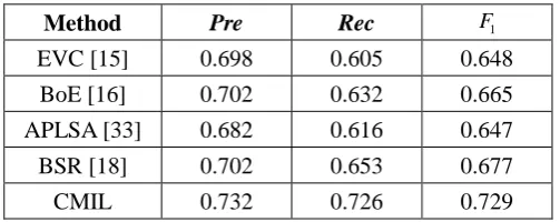
experiment, we obtained performance of each method.

Method Pre Rec F1

EVC [15] 0.698 0.605 0.648

BoE [16] 0.702 0.632 0.665

APLSA [33] 0.682 0.616 0.647

BSR [18] 0.702 0.653 0.677

CMIL 0.732 0.726 0.729

(1) CMIL vs Affective Image Classification Methods

Experimental results for the CMIL and for other general affective image classification methods are

shown in Table 3. Similar conclusions to those in the previous experiment were obtained. The

proposed CMIL method still outperforms the competing affective image classification methods.

Interestingly, we found that the precision values of these global methods are slightly higher than their

recall values. It proves that some horror images are misclassified as a non-horror because of the

background.

Table 4. Performance comparison with other MIL methods on the 10000 horror image set.

Method Pre Rec F1

mi-SVM [24] 0.657 0.695 0.675

MI-SVM [24] 0.649 0.687 0.667

miGraph [25] 0.682 0.691 0.686

MIGraph [25] 0.684 0.701 0.692

CMIL 0.732 0.726 0.729

(2) CMIL vs MIL

The experimental results of the CMIL and other MIL methods are listed in Table 4. The proposed

CMIL still outperforms the MIL methods on this larger set. The miGraph and MIGraph methods still

achieve slightly better performance than mi-SVM and MI-SVM. In addition, the precision values of

the local methods mi-SVM and MI-SVM are slightly lower than their recall values. It implies that

some non-horror images are misclassified as horror images because of their local similarity. The

precision and recall values of each contextual algorithm are comparable. It again indicates that

contextual cues are helpful for good horror image recognition scheme. When facing the larger scale

complex Internet image set, our proposed CMIL still has stable performance.

5.3

Horror Image Recognition Based on CMIL with Visual Saliency

We evaluated the proposed CMIL with improved initialization using the tensor-based visual saliency

map (denoted as CMIL+TVS). Before evaluating its performance on horror image recognition, we

including Itti’s method (Itti) [46], Hou’s method (Hou) [51], Graph-based visual saliency algorithm

(GBVS) [50], and Frequency-tuned salient region detection algorithm (FS) [52], in the context of

visual saliency map computation.

5.3.1 Comparison of Visual Saliency Maps

(1) Error Measurement for Visual Saliency Model

Given the ground truth annotation EM q( ) and the computed visual saliency SM q( ) of an

image, the precision (Spr), recall(Sre), and F_0.5 measure, which are widely used for visual saliency

map evaluation [48], were used for performance comparison:

0.5

( ) ( ) ( ) ( ) _{(1 0.5)}

, , .

( ) ( ) 0.5

SM EM SM EM _{Spr Sre}

Spr Sre F

SM EM Spr Sre

+ × ×

= = =

× +

∑

∑

∑

∑

q q

q q

q q q q

q q (18)

(2) Comparison of Visual Saliency Models

There are 3 parameters in the tensor-based saliency map model. The block size, which has little

effect because of the pyramid architecture, was set as w=8. We set dr=3 _and dc=1, meaning

that matrices U3_row, U3_column, and U1_color were used as basis for tensor reconstruction. The Precision (Spr), Recall (Sre) and F_0.5 values of each method are listed in Table 5.

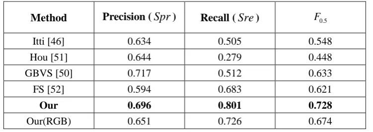
Table 5 Comparison with existing visual saliency algorithms on the 1000 horror image set

Method Precision (Spr) Recall (Sre) F0.5

Itti [46] 0.634 0.505 0.548

Hou [51] 0.644 0.279 0.448

GBVS [50] 0.717 0.512 0.633

FS [52] 0.594 0.683 0.621

Our 0.696 0.801 0.728

Our(RGB) 0.651 0.726 0.674

The performance of our tensor-based model is Spr=0.696, Sre=0.801 and F_0.5 =0.728

respectively, showing that it outperforms the other visual saliency computation methods on this set.

Because the other visual saliency methods are designed only from the visual viewpoint, they do not

consider the higher emotional stimulus in horror images. In order to test the effectiveness of the color

emotion space, we also show the tensor-based model’s results in RGB color space in Table 5 (denoted

as Our(RGB)). The lower performance from RGB space indicates that the color emotion space does

indeed identify colors with a strong emotional impact and is helpful for emotion-related salient

in the proposed tensor-based saliency map model also improve the accuracy of the saliency map. For

the qualitative comparison, some saliency maps of the horror images generated by different

algorithms are also given in Figure 8. Our proposed method correctly detects the horror regions in

almost all of these images.

Figure 8. Exemplar saliency maps on horror images produced by different algorithms.

5.3.2 Performance Comparison of Horror Image Recognition on 1000 Horror Image Set

In order to further evaluate the effect of the visual saliency map in the CMIL, we compared the CMIL

without the visual saliency map (denoted as CMIL) to the CMIL+TVS, as well as the CMIL with the

GBVS visual saliency map (denoted as CMIL+GBVS) in terms of horror image recognition. The

results are listed in Table 6. The fact that both CMIL+TVS and CMIL+GBVS outperform the CMIL

implies that the visual saliency maps do indeed give useful weak labels to the CMIL for improving its

performance on horror image recognition. In addition, the CMIL+TVS can achieve a slightly higher

1

F value than the CMIL+GBVS, it is because the GBVS has lower performance on visual salient

region detection than the proposed tensor-based model in Table 5.

Table 6. Performance comparison among different CMIL algorithms on the 1000 horror image set.

Method Pre Rec F1

CMIL 0.771 0.763 0.767

CMIL+GBVS 0.781 0.776 0.778

CMIL+TVS 0.809 0.801 0.805

5.3.3 Performance Comparison of Horror Image Recognition on 10000 Horror Image Set

We also compared the CMIL, CMIL+TVS and CMIL+GBVS methods on this larger image set.

and the CMIL.

Table 7. Performance comparison among different CMIL algorithms on the 10,000 horror image set.

Method Pre Rec F1

CMIL 0.732 0.726 0.729

CMIL+GBVS 0.731 0.733 0.732

CMIL+TVS 0.786 0.773 0.779

We gave examples of the horror region extraction results of the proposed CMIL+TVS algorithm.

Because the instance with the largest contextual score in a bag in the CMIL is most likely to evoke

horror emotion, we considered it to be a horror region in the image. Figure 9 gives some horror

region extraction results from the CMIL+TVS method. It shows that the CMIL+TVS can correctly

identify the underlying horror region of each horror image. Furthermore, the isolated horror regions

shown in the second row of Figure 9 evoke almost no feeling of horror. This again indicates that the

horror emotion expressed by an image is not evoked by an isolated region but its context.

Figure 9. Examples of horror regions extraction from the CMIL+TVS. The first row contains original images; the images in the second row are segmentation results; the images in the third row are the horror regions extracted by our CMIL algorithm.

6

Conclusions and Future Work

Considering the challenges in horror image recognition from a contextual perspective, we have

proposed a novel context-aware multi-instance learning model (CMIL). The CMIL model is based on

the fact that the emotion of horror is not evoked by isolated image regions but by the interactions

visual saliency values that are generated by the proposed tensor-based visual saliency method. The

effectiveness of our proposed CMIL framework has been validated on two large scale horror image

sets collected from the Internet. Experimental results have showed that the proposed CMIL algorithm

is superior to both general affective image classification methods and traditional MIL methods in

horror image recognition.

There is still much that has to be done in order to obtain more reliable and general horror image

filtering systems. Our future work will focus on the following directions: (1) Exploring more

effective emotion-related features for horror image recognition; (2) Integrating the image content

analysis with surrounding text tags to filter the horror content on the Web; (3) Investigating online

learning scheme so that we can dynamically adjust the classifier as more samples become available.

ACKNOWLEDGMENTS

This work was supported by the National Nature Science Foundation of China (No. 61370038,

61472421, and 61571045), the 973 Basic Research Program of China (No. 2014CB349303), the

Project Supported by CAS Center for Excellence in Brain Science and Intelligence Technology, and

Chinese National Programs for High Technology Research and Development (863 Program)

(No.2012AA012503 and No. 2012AA012504).

References

[1] W. Hu, O. Wu, and Z. Chen. Recognition of pornographic web pages by classifying texts and images. IEEE Transaction on Pattern Analysis and Machine Intelligence, 29(6): 1019-1034, 2007.

[2] M. Hammami,

Content-Based Analysis. IEEE Transaction on Knowledge and Data Engineering, pp. 272-284, 2006.

[3] A. Field, and J. Lawson. Fear information and the development of fears during childhood: effects on implicit fear responses and behavioural avoidance. Behaviour Research and Therapy, 41(11): 1277-1293, 2003.

[4] S. Rachman. The conditioning theory of fear acquisition. Behaviour Research and Therapy, 15(5):375-378, 1977.

[5] T. H. Ollendick and N. J. King. Origins of childhood fears: An evaluation of Rachman's theory of fear acquisition. Behaviour Research and Therapy, 29(2):117 -123,1991.

[6] http://en.wikipedia.org/wiki/Motion_Picture_Association_of_America_film_rating_system [7] http://slashdot.org/article.pl?sid=08/02/16/0654237

[8] http://seattletimes.nwsource.com/html/entertainment/2009687065_apeubritainhorrorfilm.html

[9] B. Wu, X. Jiang, T. Sun, S. Zhang, X. Chu, C. Shen, and J. Fan. A Novel Horror Scene Detection Scheme on Revised Multiple Instance Learning Model. Proc. International Conference on Multimedia Modeling, pp.359-370, 2011.

[10] J. Wang, B. Li, W. Hu, and O. Wu. Horror Movie Scene Recognition based on Emotional Perception. Proc. International Conference on Image Processing, pp.1489-1492, 2010.

[11] J. Wang, B. Li, W. Hu, and O. Wu. Horror Video Scene Recognition via Multiple-Instance Learning. Proc. International Conference on Acoustics, Speech, and Signal Processing, pp. 1325-1328, 2011.

[12] W. Wang, and Q. He. Survey on Emotional Semantic Image Retrieval. Proc. International Conference on Image Processing, pp. 117-120, 2008

[13] W. N. Wang and Y. L. Yu. Image emotional semantic query based on color semantic description. Proc. International Conference on Machine Learning and Cybernetics, pp. 4571-4576, 2005.