BIROn - Birkbeck Institutional Research Online
Hu, W. and Ding, X. and Li, B. and Wang, J. and Gao, Y. and Wang, F.
and Maybank, Stephen J. (2016) Multi-perspective cost-sensitive
context-aware multi-instance sparse coding and its application to sensitive video
recognition. IEEE Transactions on Multimedia 18 (1), pp. 76-89. ISSN
1520-9210.
Downloaded from:
Usage Guidelines:
Please refer to usage guidelines at or alternatively
Multi-Perspective Cost-Sensitive Context-Aware Multi-Instance Sparse
Coding and Its Application to Sensitive Video Recognition
1Weiming Hu1, Xinmiao Ding2, Bing Li1, Jianchao Wang1, Yan Gao1, Fangshi Wang3, and Stephen Maybank4 [email protected]; [email protected]; [email protected]; [email protected]; [email protected];
[email protected]; [email protected] 1
National Laboratory of Pattern Recognition, Institute of Automation, Chinese Academy of Sciences, Beijing 100190 2
Shandong Institute of Business and Technology 3
Beijing Jiaotong University, Beijing 100044) 4
Department of Computer Science and Information Systems, Birkbeck College, Malet Street, London WC1E 7HX
Abstract: With the development of video-sharing websites, P2P, micro-blog, mobile WAP websites, and so on, sensitive videos can be more easily accessed. Effective sensitive video recognition is necessary for web content security. Among web sensitive videos, this paper focuses on violent and horror videos. Based on color emotion and color harmony theories, we extract visual emotional features from videos. A video is viewed as a bag and each shot in the video is represented by a key frame which is treated as an instance in the bag. Then, we combine multi-instance learning (MIL) with sparse coding to recognize violent and horror videos. The resulting MIL-based model can be updated online to adapt to changing web environments. We propose a cost-sensitive context-aware multi-instance sparse coding (MI-SC) method, in which the contextual structure of the key frames is modeled using a graph, and fusion between audio and visual features is carried out by extending the classic sparse coding into cost-sensitive sparse coding. We then propose a multi-perspective multi-instance joint sparse coding (MI-J-SC) method that handles each bag of instances from an independent perspective, a contextual perspective, and a holistic perspective. The experiments demonstrate that the features with an emotional meaning are effective for violent and horror video recognition, and our cost-sensitive context-aware MI-SC and multi-perspective MI-J-SC methods outperform the traditional MIL methods and the traditional SVM and KNN-based methods.
Index terms: Cost-sensitive context-aware MI-SC, Multi-perspective MI-J-SC, Horror video recognition, Violent video recognition, and Video emotional feature extraction.
1. Introduction
The emergence and development of video-sharing websites, P2P, micro-blog, podcasting, mobile WAP websites, and 3GP websites facilitate the dissemination of sensitive videos, such as adult, horror, violent, and
1
terrorist videos. Fig. 1 shows some examples of violent videos and horror videos. Diffusion of sensitive videos poses a major threat to national security, social stability, and the physical, psychological, and mental health of viewers. Effective recognition of sensitive videos is necessary for web content security [54]. Recognition of sensitive videos is a newly emergent research topic in the multimedia and pattern recognition communities, in the context of multimedia retrieval [55, 56], multimedia content understanding [59, 60], and multimodal fusion [56, 57], etc. In recent years a number of specific attempts have been made to deal with the problem of sensitive video recognition, and most of them focus on adult video recognition [11, 12, 18, 21]. In this paper, we focus on recognition of horror videos and violent videos.
(a)
[image:3.595.67.532.274.457.2](b)
Fig. 1. Examples of frames taken from (a) violent videos and (b) horror videos.
1.1. Related work
Cepstral coefficients (MFCCs). Visual and audio features can be combined to more accurately locate violent scenes. Nam et al. [32] recognized violent videos by detecting blood and flames and exploiting representative audio effects, such as explosions and gunshots. Smeaton et al. [35] combined visual and audio features to select representative shots in an action video. Giannakopoulos et al. [43] detected violence using the statistics of audio features and average motion and motion orientation variance features. Lin and Wang [45] combined auditory and visual classifiers in a co-training way to detect violent shots in movies.
Horror videos strive to elicit the primary emotions of fear, horror, and terror. The contents of horror videos include serial killings, ghosts, monsters, vampires, animal killing, and irreligion. Horror information may arouse fears in children and teenagers and even induce phobias [46, 47]. The earlier work [5, 6, 8] on horror video recognition was carried out as a part of a video scene classification based on human emotions. Specific work on horror video recognition with its own characteristics emerged [13, 14]. Xu et al. [14] detected audio emotional events to locate horror video segments in videos which are known a priori to contain such segments. Wu et al. [13] represented each video as a bag of independent frames and applied multi-instance learning (MIL) to horror video recognition.
The current methods for violent and horror video recognition have the following limitations:
They focus on using low level visual, motion, and audio features, or they only use affective audio features. Research on affective color and visual semantics, together with affective audio semantics in violent and horror videos, is still exploratory, but the results of this research are available for application to violent and horror video recognition.
The current methods only focus on independent frames and do not consider the underlying contextual cues within violent and horror videos, even though contextual cues between frames are useful for recognizing violence and horror.
While contexts between frames are useful for recognizing violent and horror emotions, independent frame cues also have emotional content. The independent frame cues, contextual cues among frames, and holistic features of the entire video are different sources of information for violent and horror video recognition. Well-chosen features from different perspectives can embody a variety of discriminative information. The current violent and horror recognition algorithms do not include the fusion of multi-perspectives to improve their performance.
to update the classifiers online when new training samples are obtained.
1.2. Our work
As a variant of supervised learning, each sample for multi-instance learning (MIL) is a bag of instances instead of a single instance. Each bag is given a discrete or real-valued label. In binary classification, a bag is considered as positive if at least one instance in it is positive, and considered as negative if all its instances are negative. As a prior, a violent or horror video contains at least one violent or horror shot2, and all the shots in a non-violent or non-horror video are necessarily non-violent or non-horror. If a video is treated as a bag and a shot in the video is treated an instance in the bag, violent and horror video recognition is consistent with the framework of MIL.So, we use MIL to recognize violent and horror videos.
The most current models for MIL in common use, such as axis-parallel concepts [15], the diverse density (DD) method [25], the expectation-maximization version of diverse density (EM-DD) [27], the MI-kernel method [28], the mi-SVM and MI-SVM [19], the mi-Graph and MI-Graph [29], and the adaptive p-posterior mixture-model (PP-MM) kernel [42], are trained in batch settings, in which the entire training set is available before each training procedure begins. Babenko et al. [48] proposed an online MIL algorithm based on a boosting technique. However, this online method assumes that all the instances in a positive bag are positive. This assumption is easily violated in practical applications. Li et al [49] extended the MIL algorithm based on embedded instance selection [16, 17] to an online MIL algorithm. However, a classifier still needs to be retrained using the new samples. The citation-kNN [26] is not part of the training process. It determines the label of each test bag using the labeled bag samples nearest to the test bag and the bag samples whose nearest bag samples contain the test bag. However, the citation-kNN is sensitive to outlier samples. Sparse coding (SC) is training-free, and the model can be updated online each time the labeled sample set is updated. Furthermore, SC is not sensitive to outliers, because the sparsity regularization can suppress outliers in the sparse representation. Therefore, we combine MIL with sparse coding to form a multi-instance sparse coding (MI-SC) technique for recognizing violent and horror videos.
The contributions of our work are summarized as follows:
We extract color emotional features according to the results from psychological experiments. These color emotional features bridge the affective semantic gap to some extent. The color emotional features together with low-level visual features, motion features, and audio features are used for
2
violent and horror video recognition.
We propose a cost-sensitive context-aware MI-SC method which can make use of the context among frames in the same video and the context between visual and audio cues for violent and horror video recognition. A video is divided into a series of shots via shot segmentation and a key frame from each shot is selected. The visual feature vector of each key frame is extracted to represent the shot in which the key frame exists. An audio feature vector is extracted for the entire video. A video is represented as a bag of instances which correspond to the visual feature vectors. A graph is constructed using the key frames as nodes to represent their contextual relations. A cost-sensitive sparse coding model is constructed to represent the context between the bag of visual feature vectors and the audio feature vector. We solve the cost-sensitive context-aware MI-SC using the existing feature sign search algorithm via a mathematical transformation.
We propose a multi-perspective multi-instance joint sparse coding (MI-J-SC) method to combine information from a contextual perspective, an independent perspective, and a holistic perspective. The contexts between key frames form only a contextual perspective for violent and horror video recognition. A key frame also includes semantic meaning, so treating a video as a bag of independent instances can be considered as an independent perspective. The holistic features for the entire video can be treated as another perspective. The information from different perspectives more fully describes a video. The current MIL lacks the ability to fuse multi-perspectives. We incorporate the joint sparse coding into multi-instance classification to fuse the features from multi-perspectives, in order to obtain more accurate recognition of violent and horror videos.
The experimental results show the effectiveness of the extracted video emotion features. The results on the violent and horror video datasets show that our methods outperform the traditional MIL-based methods and the traditional SVM and KNN-based methods. The results on the general MIL datasets show that our methods may be effective for other general multi-instance problems.
2. Multi-Instance Sparse Coding
Multi-instance sparse coding (MI-SC) carries out MIL using the sparse coding technique. In the following, we first briefly introduce sparse coding. Then, we describe the mechanism of MIL via sparse coding.
2.1. Sparse coding
The goal of sparse coding [20] is to represent each input vector approximately as a weighted linear combination of “basis vectors” such that a small number of weights are non-zero. Given an h-dimensional input vector h
x and n basis vectors [ ,1 2,..., ]
h n n
U u u u , a sparse vector w n
, whose entry wj
(1 j n) is the weight of uj, is found such that
1
n j j j
w
x Uw u . (1)
The objective of sparse coding is usually formulated as the minimization of the reconstruction error with sparsity regularization:
2
2 1
min
w x Uw w (2)
where the 1 norm w1 of w is the sparsity term and λ is a regularization factor to control the sparsity of w.
2.2. MIL via sparse coding
For MIL, a training dataset {(X1,y1), , (Xi,yi), , (XN,yN)} consists of N bags { }N1 i i
X and their labels { } 1
N i i
y . A bag Xi consists of ni instances: { ,1, , , , , , }
i
i i i j i n
X x x x , where each instance xi j, is a
vector. The task of MI-SC is to sparsely combine the training bags { }N1 i i
X to represent a test bag.
Due to the set structure of the bags, a test bag cannot directly be sparsely and linearly reconstructed using the training bags. We apply a mapping function : d
X to map each bag X to a high dimensional vector space: X( )X (the descriptions and handling of the mapping functions will be detailed in Section 3.3). Then, by mapping the training bags to the high dimensional vector space, a basis matrix
1 2
[ ( ), ( ), , ( N)]
B X X X for sparse coding is obtained. Given a test bag Xt, the sparse coding in the
high dimensional vector space is defined as:
2
2 1
min ( t)
w X Bw w . (3)
representing Xt. It is clear that this is a training-free online learning model which is updated only by changing the labeled samples. The limitation of the above MI-SC is that the contexts among instances are not modeled.
3. Cost-Sensitive Context-Aware MI-SC
To handle the above limitation, we formulate context-aware MI-SC and cost-sensitive sparse coding, and propose a method for optimizing the coefficients for the cost-sensitive context-aware MI-SC.
3.1. Context-aware MI-SC
Traditional MIL usually assumes that instances in a bag are independent of each other. Zhou et al. [29] built a graph [33] in their SVM-based MIL method to model the contexts between instances in each bag. This graph representation of contexts is incorporated into our MI-SC method.
For a bag Xi, a graph Gi whose nodes are the instances in the bag is constructed. The distances between instances are computed. If the distance between two instances is smaller than a preset threshold, then the weight for the edge between the corresponding two nodes is set to 1, otherwise the weight is set to 0. A matrix Ei nini of the adjacency weights for
i
G is obtained, where i, 1
a a
E (a1, 2,...,ni).
The training samples are represented as {(X1,G y1, ),...,(1 Xi,G yi, ),...,(i XN,G yN, N)}, and a test bag is given as
(Xt,G yt, t). We apply a mapping function :G d to map each graph G to a high dimensional vector space: G( )G . Then, the basis matrix for spare coding is replaced by C[ (G1), ( G2),..., (Gn)]. The context-aware MI-SC is formulated as:
2
2 1
min (Gt)
w Cw w . (4)
3.2. Cost-sensitive sparse coding
In real applications, each bag Xi may be associated with another kind of feature. For example, an audio is usually associated with a video, and the holistic features of the audio can overall characterize the entire video. We propose a cost-sensitive sparse representation to incorporate the associated features into the bags.
For each bag Xi, its associated feature vector ai is extracted. Then, the training set can be represented by
( ,a X1 1,G y1, 1), (a X2, 2,G y2, 2),..., (aN,XN,GN,yN)
. Given a test bag Xt, we define a diagonal matrixN N
1
( t , , i t , , N t )
diag
D a a a a a a . (5) To incorporate the associated features into the MI-SC, we formulate cost-sensitive context-aware MI-SC in a high dimensional feature space as follows:
2
2 1
min (Gt)
w Cw Dw . (6)
where the diagonal matrix D is included into the 1 norm in (4). The entries in D are cost values for the different training samples. In this way, the training samples, whose associated feature vectors have small distances to the associated feature vector of the test bag, are more likely to be selected to reconstruct the test bag. In the sensitive video recognition application, the videos which have audio tracks similar to the test video are more likely to be chosen to represent the test video.
3.3. Optimization
The traditional sparse coding optimization methods cannot be directly applied to the cost-sensitive context-aware MI-SC in (6). We transform the objective function in (6) to a form to which the traditional sparse coding optimization can be applied. Then the feature sign search (FSS) algorithm is used to solve for the coefficient vector w. Let qDw, where N
q . In order to ensure that D is invertible, we add a very small value ε to the diagonal entries of D, and obtain an inverse as follows:
1 1 1
1
1 t , 2 t ,..., N t
diag
D a a a a a a (7)
Substituting -1 =
w D q into (6) yields:
2 1
1 2
min (Gt)
q CD q q . (8)
Let VCD1
, where V d N
. Formula (8) is rewritten as: 2
2 1
min (Gt)
q Vq q . (9)
The function ( ) which is used to map bags into a high dimensional space is difficult to define explicitly. Instead, the scalar product (Gi)T(Gj) in the high dimensional space is explicitly defined via a kernel function. So, we transform the objective of (9) into a form involving scalar products ( )T ( )
i j
G G
. It is clear
that
2 2
(Gt) (Gt) ] [ (T Gt) ] [ (Gt)]T (Gt) T T 2 T T (Gt)
Vq =[ Vq Vq q V Vq q V . (10)
Then, we only need to consider T
V V and T ( )
t
G
1 1 1 1
1 1
1 2 1 2
1 1 1 2 1
1 2 1 2 2 2
1 2 = ( ) = ( ) ( ), ( ),..., ( ) ( ), ( ),..., ( ) ( ) ( ) ( ) ( ) ... ( ) ( ) ( ) ( ) ( ) ( ) ... ( ) ( ) ( ) ... ... ... ... ( ) ( ) ( ) ( ) ... ( ) T
T T T
T T
N N
T T T
N
T T T
T N
T T
N N N
G G G G G G
G G G G G G
G G G G G G
G G G G G
V V CD CD D C CD
D D D 1 ( ) T N G D (11) and 1 1 1 2 1 1 2 ( ) ( ) ( ) ( ) [ ( ), ( ),..., ( )] ( ) ( ) ( ) ( ) ( ) ( ) ( ) ( )
T T T T
t t N t
T t T T t T N t
G G G G G G
G G G G G G
V CD D
D . (12)
It remains to define a graph kernel function Kg() to represent the scalar product ( ) ( )
T
i j
G G
of graphs
i
G and Gj in the high dimensional feature space. The definition of a graph kernel function depends on a kernel function between any two instances. The Gaussian radial basis function (RBF) kernel K(xi a, ,xj b, ) between an instance xi a, in bag i and an instance xj b, in bag j is defined as:
2
, , , , 2
( i a, j b) exp i a j b
K x x x x (13)
where ρ is a scaling factor. Let i a, be the weight for the instance xi a, , in bag i, which is defined as:
,
, 1
1
i
i a n
i a u u E
(14)where u is the index for an instance in bag i and i
E is the adjacency weight matrix for bag i. The kernel function g() [29] between graphs Gi and Gj is defined as:
, , , , 1 1 , , 1 1 ( , ) ( , ) j i i i n n
i a j b i a j b a b
g i j n n
i a j b
a b K G G
x x. (15)
Using the graph kernel function, the objective function in (9) is explicitly formulated, and then the optimization in (9) is efficiently solved by the recently proposed feature-sign search algorithm (FSS) [30].
3.4. Classification
the test bag belongs. For each label m, we define a vector δm N
whose l-th entry m l
is:
0
l l
m l
l
q y m
y m
,
, (16)
i.e., this vector only selects coefficients associated with labels m. The reconstruction residual m(Gt) of the test bag for label m is defined as:
2
2
( ) ( ) m 1 ( m T) T m 2( m T) T ( )
m Gt Gt Vδ δ V Vδ δ V Gt (17)
where (Gt)T(Gt)1. We assign the test bag the final label c which is defined as follows:
arg min( m( t))
m
c G .
(18)
4. Multi-Perspective Multi-Instance Joint Sparse Coding
Based on the structured joint sparse representation [2, 3, 34], we propose multi-perspective cost-sensitive MI-J-SC which includes the above cost-sensitive context-aware MI-SC.
4.1. Structured joint sparse representation
It is assumed that there are K different types of feature and M labels in the training dataset. Let
k m h N k m
Ψ be the matrix of each feature k (k=1,2,..,K) for the training samples with label m, where hk is the dimension of the k-th type of feature and Nm is the number of the training samples with label m:
1
M m
m N N
. Then, the matrix of the k-th type of feature for all the training samples is1 2
[ , ,..., ]
k k k k
M
Ψ Ψ Ψ Ψ . The k-th type’s feature vector zk hk of a test sample Z is reconstructed from the
k-th feature vectors of the training samples:
1
M
k k k k
m m
m
z Ψ w (19)
where k Nm m
w is the reconstruction coefficient vector for the k-th feature vectors of the samples with label
m, and k is the residual term. Let ( 1) , ( 2) ,..., ( )
T
k k T k T k T N
M
w w w w be the coefficient vector for the
k-th type of feature. Let W[w w1, 2,...,wK] N K . The
2,1-mixed norm of W is: 2
2,1 2 2
1 1 1
M K M
k
m m
m k m
W w W (20)
where 1 2
[ , ,... K] Nm K
m m m m
regression based on the 2,1 mixed- norm regularization [2, 3, 34]: 2
2,1
1 1 2
1 min
2
K M
k k k
m m
k m
W z Ψ w W . (21)
The 2,1 mixed-norm includes the 2 norm of the vector of the coefficients of the K feature vectors for each training sample and the 1 norm of the vector of the 2 norm values for all the samples. The 2,1 mixed-norm guarantees joint sparse representation. The reasons are summarized as follows:
The 1 norm in the 2,1 mixed-norm ensures that the training samples chosen to represent a test
sample are as few as possible.
The 2 norm in the 2,1 norm ensures that when a training sample is not chosen to represent a test
sample, all the K feature vectors of the training sample are not chosen to represent the test sample. This structured joint sparse coding can effectively fuse information from multiple features.
4.2. Multi-perspectives of multi-instances
We extend the above structured joint sparse representation to MIL to fuse information from multi-perspectives. Different perspectives can be defined according to different applications. We define the following three multi-perspectives in the context of sensitive video recognition:
1) Independent perspective: As in traditional MIL, the instances in a bag are treated as independent. We define a mapping function 1
:X d1 to map the feature space of the bags { }X to a
1
d -dimensional vector space: X1( )X . Then, the training samples are transformed to F1[1(X1), ,1(Xi), ,1(XN)].
In the d1-dimensional vector space, we define a kernel function 1() between any two bags Xi and Xj
as follows:
1 1 1 1
1
1 1 1 1
( , ) ( , ) [ ( )] ( )
( , ) ( , )
j i
j j i i
n n
ia jb
T a b
i j i j n n n n
il il js js
l l s s
K
K K
x x
X X X X
x x x x
(22)
where the kernel K() between two instances is defined as in (13).
2) Contextual perspective: The graph constrained MI-SC in Section 3.1 is introduced to form a contextual perspective for MIL. We define a mapping function 2
:G d2 to map the features of each bag
bags are transformed to 2 2 2 2 1
[ (G), , (Gi), , (GN)]
F . In the d2-dimensional vector space, the kernel function 2() is defined as in (15).
3) Holistic perspective: Statistical histograms of instances in bags can be used for bag classification. From a holistic perspective, we construct a feature histogram for a bag based on the bag-of-words model [4]. Given the set of the training bag samples, all the instances are clustered to form a lexicon of R code words
1
{ ,d ,dr,...,dR}. Each instance xij in a bag Xi is mapped to a code word (xij) which is determined by:
1
( ij) arg min ij r
r R
x x d . (23)
In bag Xi , the number of occurrences h r( ,Xi) of each code word r (r1, 2,...,R) is counted:
( , i) { ij i: ( ij) }
h r X x X x r , where | | is the number of entries in a set. Then, bag Xi is represented by a normalized histogram ξi:
1 1 1
(1, ) ( , ) ( , ) , , , ,
( , ) ( , ) ( , )
i i i
i R R R
i i i
r r r
h h r h R
h r h r h r
X X X
ξ
X X X
. (24)
Then, the set of the training samples is represented by {(X ξ1, ,1 y1), , (X ξi, ,i yi), , (XN,ξN,yN)}. We map each histogram feature vector to a high dimensional feature space using a mapping function 3
: d3
i
ξ .
Then, the histograms of the training samples are transformed to F3[3( ),...,ξ1 3( ),...,ξi 3(ξN)]. In this high
dimensional space, we define the kernel function between any two bags as follows:
1 2
1 2
3 3
3 1 2
1 1
( , ) [ ( )] ( ) [ ] [ ] ( , )
R R
T
i j i j i j r r
r r
r r K
ξ ξ ξ ξ
ξ ξ d d (25)where
1 2
( r, r)
K d d is the Gaussian kernel function between two code words
1
r
d and
2
r
d :
1 2 1 2
2 ( r, r) exp( r r )
K d d d d . (26)
4.3. Multi-perspective cost-sensitive MI-J-SC
We use the structured joint sparse representation in Section 4.1 to fuse the information from multi-perspectives such as defined in Section 4.2. Also, cost-sensitive sparse coding can be applied to the structured joint sparse representation. Then, we propose a multi-perspective cost-aware MIL method by integrating multi-perspectives into a unified joint sparse coding framework based on the 2,1 norm. Given K
perspectives (K is 3 in this paper), the training sample set is represented by K matrices 1 2 { , ,..., K}
1 2
[ ( ), ( ),..., ( )]
k k k k
N
F X X X . Given a test sample Xt , its feature vector in each perspective k is represented by fk k(Xt). Let
k N
w be the coefficient vector for the training samples at perspective k
and W be the matrix of the coefficient vectors of the K perspectives: 1 2
[ , ,..., K] N K
W w w w . Then, multi-perspective cost-sensitive MI-SC is represented by:
2 2,1 2 1 1 min 2 K
k k k
t k
W f F w DW (27)
where D is the cost matrix defined in (5). In (27), the first term is the sum of the squared reconstruction errors from different perspectives, and the second term is the regularization to control the sparsity of the coefficients. We group the training feature set k
F of each perspective k according to the class labels { }M1 m
m of the training samples: k [ 1k,..., k,..., k]
m M
F F F F where k m
F is the matrix which consists of the k-th feature vectors of the training samples with label m. Accordingly, the k-th coefficient vector in W is also grouped as:
1
( k T) ,..., ( k) ,..., (T k )T T
m M
w w w . Let [ 1, 2,..., K] Nm K
m m m m
W w w w (m=1,2,..,M), where Nm is the number of the training samples with class m. Then, Equation (27) is rewritten as:
2
2,1
1 1 2 1
1 min
2
K M M
k k k
t m m m m
k m m
W f F w D W (28)
where Nm Nm m
D is the diagonal matrix whose entries are those elements in D corresponding to the training samples with label m.
4.4. Optimization
The 2,1 mixed-norm accelerated proximal gradient (APG) algorithm [34] is introduced to optimize the object function in (28). The APG cannot be directly applied to (28). We make a transformation to (28). Let
m m m
Q D W where 1 2
[ , ,..., K] Nm K
m m m m
Q q q q . 1
m m m
W D Q . 1
( )
k k k k
m m m m m
F w F D q . Let 1
( )
k k
m m m
U F D . It follows that (28) is equivalent to:
2
1 1 1
1 min
2
K M M
k k k
t m m m
k m m
2 W 2f U q Q . (29)
The APG algorithm can be applied to (29).
The APG algorithm alternately updates a coefficient matrix t [ k t, ]
m
Q q and an aggregation matrix ,
[ ]
t k t
m
In the generalized gradient mapping step, given the current aggregation matrix ˆt
V , the coefficient matrix t
Q is updated. Let Uk [U1k,...,Ukm,...,UMk ]. It is clear that
1 1 1 2 1
1 2 1 2 2 2 1
1 2 ( ) ( ) ( ) ( ) ... ( ) ( ) ( ) ( ) ( ) ( ) ... ( ) ( ) ( ) ... ... ... ( ) ( ) ( ) ( ) ... ( ) ( )
k T k k T k k T k
N
k T k k T k k T k
T T N
k k
k T k k T k k T k
N N N N
X X X X X X
X X X X X X
U U D D
X X X X X X
(30) and 1 1 2 ( ) ( ) ( ) ( ) ( ) ( ) ... ( ) ( )
k T k
t
k T k
T k T t
k t
k T k
N t X X X X
U X D
X X
(31)
where the scalar product k(Xi)Tk(Xj) between bags Xi and Xj is evaluated using a kernel function
which is explicitly defined in (15), (22), or (25). A matrix Pt [p1,t,...,pk t,,...,pK t, ] N K is defined as
follows:
, ( ) ,
k t T T k t
k t k kv
p U X U U , k=1,2,..,K. (32) Then,
, 1 , ,
k t k t k t
q v q , k=1,2,…,K (33) and
1 1
1 2
max 1 ,0 , 1, ,
t t
m t m
m m M q q
q (34)
where is the step size parameter.
In the aggregation step,the aggregation matrix is updated by constructing a linear combination of t
Q
and t1
Q :
1 1 1(1 ) 1
( )
t t t t t t
t
V Q Q Q (35)
where conventionally t 2 / (t2) [36].
4.5. Classification
22
1 1
( ) ( ) ( ( )) ( ) ( ) 2( ) ( ) ( )
K K
k k k k T k T k k k T k k
m t t m m m m t m
k k
K
X X U q δ q U U δ q U X δ q (36)
where ( k)
m
δ q is a coefficient selector that only selects coefficients associated with label m, i.e., the l-th
entry in ( k)
m
δ q is defined as follows:
( ) 0
l l
k
m l
l
q y m
d
y m
q ,
, . (37)
[image:16.595.196.406.270.510.2]Similar to (18), the label that has the smallest residual is assigned to the test bag Xt.
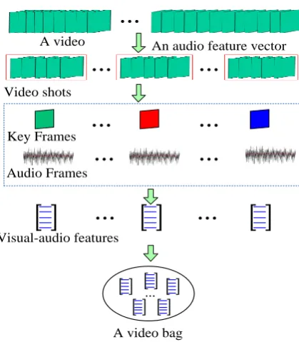
5. Sensitive Video Recognition
Fig. 2. Bag construction for each video.
We apply the proposed cost-sensitive context-aware MI-SC and multi-perspective MI-J-SC to recognize sensitive videos, especially horror videos and violent videos. Given a set of N videos { ,I I1 2,...,IN}, they are labeled as { ,y y1 2,...,yN} (yi{1, 2}, i.e., M=2) where a sensitive video is labeled “1” and a non-sensitive
video is labeled as “2”. Each video Ii is divided into ni shots {si,1,si,2,...,si n,i} by measuring mutual
information and joint entropy between frames [37]. In each shot, we select the frame which is closest to the mean of the color emotional features in the shot as a key frame, and then a key frame set { ,1, ,2,..., , }
i
i i i n
θ θ θ for
video Ii is obtained. The visual and audio feature vector fi j, for each key frame θi j, is extracted. An audio feature vector ai is extracted from the entire audio associated with Ii. A bag for each video is constructed
by treating the feature vector of each key frame as an instance, as shown in Fig. 2. Then, the above MI-SC
A video
Video shots
Key Frames Audio Frames
Visual-audio features
A video bag
...
...
...
...
...
...
...
...
...
...
methods can be applied to { ,I I1 2,...,IN}. The optimal coefficients obtained by the cost-sensitive context-aware MI-SC or the multi-perspective MI-J-SC are used to classify the test videos as sensitive or non-sensitive. In the following, we describe the features extracted from horror and violent videos.
The features extracted from videos are based on emotional perception theory. Different colors, textures, and audio rhythms may produce different emotions. So, we extract the following video features that produce emotions in the viewers: color emotional features, visual features, and audio features. These emotion-producing features are used for horror video recognition. Additional motion features are used for recognizing violent videos.
5.1. Color emotional features
Ou et al. [38, 39] developed color emotion models for single colors and harmony models for two color combinations by psychophysical experiments. We extract color emotional features based on these color emotion models.
Ou et al. found that color emotions for single-colors depend on the following three factors: activity, weight, and heat, which are defined as follows:
* 2 * 2 * 2
* 0
* 1.07 0
2.1 0.06 ( 50) ( 3) (( 17) / 1.4) 1.8 0.04(100 ) 0.45cos( 100 )
0.5 0.02( ) cos( 50 )
Activity L a b
Weight L h
Heat C h
(38)
where ( * * *
, ,
L a b ) and ( * *
, ,
L C h) are the color components in the CIELAB and CIELCH color spaces, respectively. Based on (38), we define an emotional intensity (EI) for each pixel (x,y) as follows:
2 2 2
( , )
EI x y Activity Weight Heat . (39) Given a frame in a video, the EIs for all the pixels are computed. Based on the EIs, a color emotion histogram is acquired and employed as part of the color emotional features.
Ou and Luo [1] developed a quantitative two-color harmony model which consists of three independent color harmony factors: hue effect (HH), lightness effect (HL), and chromatic effect (HC). These three harmony factors for two colors are explicitly estimated using hues, saturations, and lightness values of these two colors in the CIELAB color space (The details can be found in [1]). The overall harmony score CH
between these two colors is defined as the sum of the three factors: CHHHHCHL. Given a frame, for
each pixel we calculate the color harmony score CH1 between its color and the mean of the colors of its
pixels in the frame. The color harmony score CHf of this pixel is defined as the sum of the two scores: CHf
=CH1+CH2. Based on the color harmony scores in the frame, we construct a color harmony histogram which
is used as another part of the emotional features.
5.2. Visual features
The visual emotional features include lighting features, color features, texture features, and Rhythm features.
1) Lighting feature: Lighting affects viewers’ feelings directly [5, 7]. The lighting effect is determined by two factors: the general level of light and the proportion of shadow area. We use the median of the L values of all the pixels in a frame in the Luv color space [7] to characterize the general level of the light in the frame. The proportion of the pixels, whose lightness values are below a certain shadow threshold, is used to estimate the proportion of shadow area.
2) Color feature: The color values used in the HSV space are clearly distinguishable by human perception, so we use the means and variances of components of the HSV color space in a frame to characterize the main cues of colors in the frame. Particular colors have strong relations with movie genres [7]. The particular colors in a frame can be represented by the covariance matrix Θ of the L, u, v values of pixels in the frame:
2 2 2
, ,
2 2 2
, ,
2 2 2
, ,
L L u L v
L u L u v
L v u v v
Θ
.
(40)The determinant of (40), det( )Θ , is used as the feature for the particular colors.
3) Texture feature: Texture is another important factor relevant to image emotion, because different textures give people different feelings. Geusebroek and Smeulders [40] proposed a six-stimulus basis for stochastic texture perception: Texture distributions in image scenes conform to a Weibull distribution associated with a random variable x:
1 1
( )
x
x
wb x e
(41)
4) Rhythm feature: In horror and violent videos, quick shot switching and strong motions are often used to excite nervous moods in the viewers. We use the inverse length of a shot to represent the speed of shot switching. For a frame, the mean and standard deviation of motions between frames in a short clip centered at the frame are used to measure the quantity of motion associated with the frame [10].
5.3. Audio features
Specific sounds and music are often used to highlight emotional atmosphere and promote dramatic effects. The following audio features [9] are extracted:
The mean and variance of the 12 MFCCs (Mel-frequency Cepstral coefficients) of each frame and the 12 MFCCS’ first-order differential, where the MFCCs are computed from the fast Fourier transform (FFT) power coefficients.
Spectral power which is used to measure the energy intensity of an audio signal: For an audio signal
s(t), each frame is weighted with a Hamming window h(t), where t is the index of a sample in the frame. The spectral power of an audio frame of the signal s(t) is calculated as:
2 1
0
1
10 log ( ) ( ) exp 2
T
t
to s t h t j
T T
(42)
where T is the number of samples of each frame, and o is the index of an order of the DFT coefficients.
The mean and variance of the spectral centroids of the audio signal, which are employed as measures of music brightness.
Time domain zero crossings rate which provides a measure of the noisiness of an audio signal.
5.4. Motion features
The following motion features are extracted especially for violent video recognition:
1) Optical flow: Corners in the previous frame are detected. Optical flow is used to estimate the positions of the corners in the current frame. The distance moved by each corner between the previous and current frames is calculated. The sum, mean, and standard deviation of the distances moved by the corners are used as motion features.
are calculated and used as additional motion features.
Empirically, all the above color emotional features, visual features, and audio features are useful for both horror video recognition and violent video recognition. The above motion features are useful only for violent video recognition, rather than horror video recognition, because violent videos use much more intense motions than horror videos to trigger strong emotions. In each instance the used features are combined into a feature vector. The value of each component in a feature vector is normalized according to the maximum of the values of this component over all the samples in the dataset. For the cost-sensitive context-aware MI-SC, all the audio features extracted from an entire video form a single audio feature vector for the video. This audio feature vector is used to calculate the cost matrix. For the multi-perspective MI-J-SC, the same features are used in all the three perspectives.
6. Experiments
In the experiments, the color emotion histogram has 64 bins. The color harmony histogram has 25 bins. The shadow threshold for lighting feature extraction was experimentally determined as 0.18. For an audio signal, we extracted a single-channel audio stream at 44.1 KHz and computed 12 MFCCs over 20ms frames.
We used the precision (P), recall (R), and F1-measure (F1) to evaluate the performance of an algorithm.
Let HS be the horror or violent videos in a dataset, and ES be the videos that are recognized as horror or violent by the algorithm. The precision (P), recall (R), and F1-measure (F1) are defined as:
1 2
HS ES
P
ES
HS ES
R
HS
P R
F
P R
(43)
The proposed sensitive video recognition methods were compared with the following methods:
EM-DD [27]: This is an MIL method which combines the EM algorithm with the diverse density (DD) maximization [25].
mi-Graph [29]: This method uses a graph [33] to model the contexts between instances in a bag. MI-kernel [28]: This method regards each bag as a set of feature vectors and then applies a
set-based kernel directly for bag classification.
mi-SVM: It looks for the hyper-plane such that for each positive bag there is at least one instance lying in the positive half-space, and all the instances belonging to negative bags lie in the negative half-space.
Citation-KNN: It is extended from KNN to deal with MIL problems. It considers not only the labels of the bags which are nearest to the test bag, but also the labels of the bags whose nearest samples contain the test bag.
SVM: The feature vectors of the key frames in a video were averaged into one vector. These averaged feature vectors of all the training samples were used to construct a classical SVM-based sensitive video classifier.
KNN: The KNN, instead of the SVM in the SVM-based classifier, was used to train a classifier. In the following, we report first the results of horror video recognition, then the results of violent video recognition, and finally the results on the general MIL datasets for validating the effect of proposed MI-SC methods.
6.1. Horror video recognition
We downloaded horror and non-horror videos from the internet. This dataset consists of 400 horror videos and 400 non-horror videos. These videos come from different countries, such as China, US, Japan, South Korea, and Thailand. The genres of the non-horror movies include comedy, action, drama, and cartoon. Half of the horror videos and half of the non-horror videos were used for training, and the remaining videos were used for testing. The average accuracies of ten times 10-fold cross validation were used to measure the performance of each method.
Table 1 shows the values of the average Precision (P), Recall (R) and F1 measure (F1) of our methods
competing methods in which the audio features are used. Therefore, we removed the audio features from the feature vectors and compared the method based on the pure context-aware MI-SC with the mi-Graph-based method without audio features. From Table 1, the following points were revealed:
Table 1. The experimental results on the horror video dataset (%)
Algorithms Precision (P) Recall (R) F1 measure Multi-perspective cost-sensitive MI-J-SC 85.56(±0.51) 85.21(±0.39) 85.38(±0.32)
Cost-sensitive context-aware MI-SC 81.62(±0.72) 83.38(±0.87) 82.46(±0.19) Pure context-aware MI-SC 80.02(±1.08) 82.00(±0.76) 80.98(±0.53) miGraph with audio features 81.87(±1.95) 82.4(±1.25) 82.14(±1.20) miGraph without audio features 80.01(±1.59) 80.82(±0.92) 80.40(±1.06) MI-kernel 80.70(±1.42) 81.43(±0.9) 81.05(±0.5)
MI-SVM 79.78 78.92 79.35
Citation-KNN 78.85 70.54 74.46
EM-DD 77.59 72.97 75.21
SVM 75.41 75.41 75.41
kNN 89.10 57.30 69.70
Our method based on multi-perspective cost-sensitive MI-J-SC is much more accurate than all the other methods. This shows that horror video recognition benefits from multi-perspectives. The lower standard deviations imply that our method is stable.
The method based on the cost-sensitive context-aware MI-SC has a higher mean F1 value and a much lower standard deviation than the method based on the pure context-aware MI-SC. This indicates that the visual-audio context is useful for horror video recognition and the method based on the cost-sensitive MI-SC effectively fuses the visual and audio features.
Our method based on cost-sensitive context-aware MI-SC, our method based on multi-perspective cost-sensitive context-aware MI-J-SC, the method based on the pure context-aware MI-SC and the method based on the mi-Graph method, all of which model contextual cues among instances in a bag, outperform other MIL-based methods in which the instances are treated independently. This shows that the contextual relations between instances are useful for horror video recognition. The results of the mi-Graph-based MIL method, in which SVMs rather than sparse coding are used,
features. It is apparent that the sparse coding-based MIL methods outperform the SVM-based MIL method for horror video recognition.
The two non-MIL-based methods, the KNN-based method and the pure SVM-based method, overall yield less accurate results than the MIL-based methods. This is because they use holistic features in videos. If a horror video contains only a small number of horror frames, then the holistic features inevitably weaken the features obtained from the horror frames. The pure SVM-based method outperforms the KNN-based method, because SVM considers experiential risk and structural risk. Furthermore, the training free characteristic of the sparse coding classifiers makes it feasible to extend our methods based on cost-sensitive context-aware MI-SC and multi-perspective cost-sensitive context-aware MI-J-SC to online classifiers that are necessary for network video analysis applications.
[image:23.595.197.398.516.642.2]The computational efficiency of the proposed model is ensured by the efficient optimization methods for obtaining the sparsity coefficient vector. The feature sign search (FSS) algorithm in the cost-sensitive context-aware MI-SC produces a significant speedup for sparse coding. The APG algorithm in the multi-perspective cost-sensitive MI-J-SC is a fast algorithm for solving the 2,1 norm-regularized optimization. Table 2 compares the runtimes of the proposed methods and other representative methods on the horror video dataset tested on a computer with Intel(R) Core(TM)2 Quad CPU. It is seen that the test speed of our sparse coding-based methods is comparable to other representative methods, not taking into account the fact that our methods have no training time.
Table 2. Runtime in seconds per video for different methods Training Test Multi-perspective
cost-sensitive MI-J-SC 0 0.07 Cost-sensitive context-aware
MI-SC 0 0.05
mi-Graph 1.02 0.05 mi-kernel 1.02 0.06 SVM 1.06 0.04 Citation-kNN 0 0.19
the combination of the visual features, the audio features, and the color emotional features can improve the recognition accuracy, which shows the complementary characteristics of the three types of features.
Table 3. The results for different feature combinations (%)
VF EF AF VF+EF VF+AF EF+AF VF+EF+AF Multi-
perspective MI-J-SC
Precision 70.1 69.8 81.0 68.8 81.6 84.1 85.4 Recall 72.7 73.6 81.8 70.4 81.3 84.7 85.2 F1 measure 71.4 71.7 81.4 69.6 81.5 84.4 85.3
mi-Graph
Precision 69.1 69.9 80.8 76.4 82.7 82.7 84.0 Recall 68.8 68.5 81.3 77.0 81.5 84.8 83.0 F1 measure 68.9 69.2 81.0 76.7 81.8 83.7 83.5
MI-SVM
Precision 72.2 73.3 71.3 72.0 84.1 81.0 80.7 Recall 73.3 74.3 81.7 74.0 83.3 81.8 82.8 F1 measure 72.8 73.8 81.5 73.0 83.7 81.4 81.8
SVM
Precision 72.8 70.6 76.9 71.0 77.4 75.6 78.6 Recall 73.0 70.3 76.5 71.5 77.0 76.5 79.0 F1 measure 72.9 70.5 76.7 71.3 77.2 76.1 78.8
kNN
Precision 76.6 72.9 86.0 74.5 88.0 89.4 89.1 Recall 58.0 71.3 50.5 57.0 49.5 57.0 57.3 F1 measure 66.0 72.1 63.6 64.6 63.4 69.6 69.7
6.2. Violent video recognition
Table 4. The experimental results on the violent video dataset (%)
Algorithms Precision (P) Recall (R) F1 measure Multi-perspective cost-sensitive MI-J-SC 86.57(±0.48) 87.87(±0.87) 87.2(±0.53)
Cost-sensitive context-aware MI-SC 86.13(±0.98) 85.95(±0.95) 86.04(±0.87) mi-Graph 85.95(±2.28) 85.82(±1.69) 85.85(±1.15) MI-kernel 84.77(±3.37) 84.99(±2.84) 84.79(±1.25)
MI-SVM 82.75 82.54 82.64
Citation-KNN 78.88 83.33 81.04
EM-DD 71.01 84.52 77.17
SVM 82.25 79.66 80.93
kNN 80.78 73.59 77.02
[image:24.595.125.472.397.562.2]more accurate results than our cost-sensitive context-aware MI-SC method. The results have the same characteristics as on the horror dataset.
[image:25.595.154.443.401.505.2]We also tested performance of violent video recognition methods on the VSD (violent scene detection) 2014 dataset [62], which benchmarks violence detection in Hollywood movies at the MediaEval benchmarking initiative for multimedia evaluation. The training set in the dataset has 24 Hollywood movies and contains binary annotations of all the violent scenes, where a scene was identified by its start and end frames. A set of 7 Hollywood movies was used for testing. All the test violent segments were annotated at video frame level, i.e., a violent segment was defined by its starting and ending frame numbers. We segmented the test videos into scenes and labeled the scenes as violent or non-violent using the videos’ annotations at the frame level. Table 5 compares the results of our methods for detecting violent scenes with the state-of-the-art results on the dataset. It is seen that the results of our methods are better than the stat-of-the-art results. The effectiveness of the extracted features and the MI-SC-based classification in our methods is clearly shown.
Table 5. Comparison between the results (%) of our methods and the state-of-the-art results on the Hollywood movie test set and the YouTube movie test set, respectively
Test subset Method Precision Recall F1 measure
Hollywood movies
Multi-perspective MI-J-SC 63.8 69.8 66.6 Context-aware MI-SC 50.8 69.5 58.7 FUDAN [63] 41.1 72.1 52.4 RECOD [61] 33.0 69.7 44.8 VIVOLAB [58] 38.1 58.4 46.1
6.3. MIL datasets
100 positive and 100 negative bags.
Table 6. Accuracy (%) on the MIL benchmark datasets
Algorithm Musk1 Musk2 Elephant Fox Tiger Multi-perspective MI-J-SC 91.1(±2.8) 90.6(±1.3) 88.5(±1.1) 62.7(±1.8) 86.8(±1.2)
mi-Graph 88.9(±3.3) 90.3(±2.6) 86.8(±0.7) 61.6(±2.8) 86.0(±1.6) MI-Graph 90.0(±3.8) 90.0(±2.7) 85.1(±2.8) 61.2(±1.7) 81.9(±1.5) MI-Kernel 88.0(±3.1) 89.3(±1.5) 84.3(±1.6) 60.3(±1.9) 84.2(±1.0)
MI-SVM 77.9 84.3 81.4 59.4 84.0 mi-SVM 87.4 83.6 82.0 58.2 78.9
Miss-SVM 87.6 80.0 N/A N/A N/A
PP-MM 95.6 81.2 82.4 60.3 82.4
DD 88.0 84.0 N/A N/A N/A
EM-DD 84.8 84.9 78.3 56.1 72.1
We compared our multi-perspective context-aware MI-J-SC method with the methods based on mi-Graph, MI-Graph, MI-Kernel, MI-SVM, mi-SVM [19], Miss-SVM [41], PP-MM kernel[42], the diverse density (DD) [25], and EM-DD [27]. For all the methods the same features from the benchmark datasets were used. The performance of each method was evaluated using the accuracy which is the proportion of the samples which are correctly classified. Our multi-perspective context-aware MI-J-SC method and the methods based on mi-Graph, MI-Graph, and MI-Kernel were run by us. The 10-fold cross validations for ten times were carried out to yield the average accuracies and standard deviations. The results of the competing methods based on MI-SVM and mi-SVM [19], Miss-SVM [41], PP-MM kernel[42], DD [25], and EM-DD [27] were directly taken from [29]. All the results are shown in Table 6. It is seen that our multi-perspective MI-J-SC method achieves better performances than the methods based on MI-Graph and mi-Graph on the Musk1, Elephant and Fox datasets. The performances of the methods based on multi-perspective MI-J-SC, MI-Graph, mi-Graph, and MI-Kernel on the Musk2 and Tiger datasets are comparable. More importantly, our multi-perspective MI-J-SC method yields lower standard deviations on all the benchmark datasets. This shows the stability of our multi-perspective context-aware MI-J-SC method.