A c o s t-s e n si tiv e d e ci sio n t r e e
l e a r ni n g a l g o ri t h m b a s e d o n a
m u l ti-a r m e d b a n d i t f r a m e w o r k
Lo m a x, S a n d Vad e r a , S
h t t p :// dx. d oi.o r g / 1 0 . 1 0 9 3 / c o mj nl/ bx w 0 1 5
T i t l e A c o s t-s e n s i tiv e d e ci sio n t r e e l e a r n i n g al g o r i t h m b a s e d o n a m u l ti-a r m e d b a n d i t f r a m e w o r k
A u t h o r s Lo m a x, S a n d Vad e r a , S
Typ e Ar ticl e
U RL T hi s v e r si o n is a v ail a bl e a t :
h t t p :// u sir. s alfo r d . a c . u k /i d/ e p ri n t/ 3 8 1 1 8 /
P u b l i s h e d D a t e 2 0 1 6
U S IR is a d i gi t al c oll e c ti o n of t h e r e s e a r c h o u t p u t of t h e U n iv e r si ty of S alfo r d . W h e r e c o p y ri g h t p e r m i t s , f ull t e x t m a t e r i al h el d i n t h e r e p o si t o r y is m a d e f r e ely a v ail a bl e o nli n e a n d c a n b e r e a d , d o w nl o a d e d a n d c o pi e d fo r n o
n-c o m m e r n-ci al p r iv a t e s t u d y o r r e s e a r n-c h p u r p o s e s . Pl e a s e n-c h e n-c k t h e m a n u s n-c ri p t fo r a n y f u r t h e r c o p y ri g h t r e s t r i c ti o n s .
CSDT learning using Multi-Armed Bandits
1
A Cost-Sensitive Decision Tree Learning Algorithm
based on a Multi-Armed Bandit Framework
Author version of paper accepted by The Computer Journal, Oxford University Press, March 2016
Susan Lomax and Sunil Vadera*
University of Salford, The Crescent, Salford, UK, M5 4WT
*corresponding author [email protected], 0161 295 5262
This paper develops a new algorithm for inducing cost-sensitive decision trees that is inspired by the multi-armed bandit problem, in which a player in a casino has to decide which slot machine (bandit) from a selection of slot machines is likely to pay out the most. Game Theory proposes a solution to this multi-armed bandit problem by using a process of exploration and exploitation in which reward is maximized. This paper utilizes these concepts to develop a new algorithm by viewing the rewards as a reduction in costs, and utilizing the exploration and exploitation techniques so that a compromise between decisions based on accuracy and decisions based on costs can be found. The algorithm employs the notion of lever pulls in the multi-armed bandit game to select the attributes during decision tree induction, using a look-ahead methodology to explore potential attributes and exploit the attributes which maximizes the reward. The new algorithm is evaluated on fifteen datasets and compared to six well-known algorithms J48, EG2, MetaCost, AdaCostM1, ICET and ACT. The results obtained show that the new multi-armed based algorithm can produce more cost-effective trees without compromising accuracy. The paper also includes a critical appraisal of the limitations of the new algorithm and proposes avenues for further research.
2
1 INTRODUCTION
Decision trees are a natural way of presenting a decision-making process, because they are simple and easy for anyone to understand [1]. Learning decision trees from data however is more complex, with most methods based on an algorithm known as ID3 which was developed by [1, 2, 3]. ID3 takes a table of examples as input, where each example consists of a
collection of attributes, together with an outcome (or class) and induces a decision tree, where each node is a test on an attribute, each branch is the outcome of that test and at the end are leaf nodes indicating the class to which an example, when following that path, belongs. ID3, and a number of its immediate descendants, such as C4.5 [4], CART [5] and OC1 [6] focused on inducing decision trees that maximized accuracy.
However, several authors have recognized that in practice there are costs involved [5, 7, 8, 9]. For example, it costs time and money for blood tests to be carried out [10]. In addition, when examples are misclassified, they may incur varying costs of misclassification depending on whether they are false negatives (classifying a positive example as negative) or false positives (classifying a negative example as positive). This has led to many studies which develop algorithms that aim to induce cost-sensitive decision trees.
3 authors have recognized that there can be a trade-off between accuracy and minimizing cost [12, 13] or a reduction in performance [14].
The survey carried out by [11] reveals there are two major approaches used to induce cost-sensitive decision trees; methods that adopt a greedy approach that aims to induce a single tree, and non-greedy approaches that generate multiple trees. Over 50 cost-sensitive
algorithms have been identified and a taxonomy developed which classifies these algorithms into seven classes by the way in which costs have been introduced.
Given such a wide range of algorithms, which one performs well? In [12] the authors carried out an independent empirical evaluation over a range of cost matrices for the following algorithms: EG2 [15], CS-ID3 [16, 17], IDX [18], MetaCost [19], MetaCost_A and
MetaCost_CSB [14], AdaCost [20], SSTBoost [21], CS-AdaBoost and CSB [14], LS-ID3, CS-LSID3 [22], and ICET [8].
The evaluation, together with the survey, lead to the following conclusions [11, 12]:
Problems arise from an imbalance in the class distribution, with most decision tree learners biasing outcomes towards the dominant class; if this class is not the most costly, this explains the reduction of accuracy rates
Multi-class datasets cause problems because the frequency of examples in each class may not be high making it difficult to distinguish between the classes; the classes themselves may be similar also. Additionally multi-class datasets have the
characteristics of imbalanced datasets
4 Trade-offs between high misclassification costs usually result in the accuracy rate
being sacrificed; the higher the misclassification costs, the more unbalanced the class distribution, the lower the accuracy rate
The nature of datasets could account for these discrepancies and inconsistent performances and one direction of research is to develop recommender systems for advising which
algorithm to use given the characteristics of the data, such as skew, number of attributes, etc. The STATLOG project [23] supported by the European Commission (ESPRIT 5170) initiated work in this direction but focused on accuracy and has continued in the EU funded project e-Lico1. A related direction of work, known as landmarking, is to use simpler learning
algorithms, such as Naive Bayes to predict the performance of other, more complex algorithms such as neural networks and support vector machines [24, 25, 26]. This line of research is interesting and has its own challenges such as how best to learn about learning algorithms, and selection of datasets to provide as training data. In contrast, this paper focuses more directly on the above issues, and aims to utilize game theory for handling the cost versus accuracy trade-off in decision tree induction.
A key feature of game theory is its ability to handle trade-offs [27, 28, 29]. Game theory can be used to predict outcomes by choosing strategies according to and linked with ‘payoffs’. The pay-offs vary but can easily be described as ‘costs’. For example in cost-sensitive learning the goal is to reduce costs, therefore the pay-off is simply the reduction of cost or to obtain the lowest cost as possible.
Cost-sensitive decision tree learning involves building a model in a cost-effective way. From examination of games and Game Theory, the Multi-Armed Bandit game looks the most promising in that its lever pulls could be viewed as generating models, and could be mapped to paths contained in a decision tree model.
1 An e-Laboratory for Interdisciplinary Collaborative Research in Data Mining and Data-Intensive Science, an
5 Cost-sensitive learning could be thought of as involving two decision-makers because there is an algorithm and costs which sometimes work together well and sometimes do not. For example, player 1; ‘accuracy-based player’ chooses strategies concentrating only on accuracy and player 2; ‘cost-based player’ chooses strategies which consider costs in some way, each produces a different set of strategies. Conflict between decisions based on accuracy and decisions based on costs require a trade-off, so a technique which deals in trade-offs should be utilized in a framework for cost-sensitive learning. What can be surmised at this stage is that the pay-offs matter when deciding strategies.
Hence, this research aims to utilize game theory as a basis for developing a cost-sensitive decision tree algorithm, which aims to address the trade-off between accuracy and cost that has been observed in previous studies.
The rest of the paper is organized as follows. Section 2 presents the background to decision tree learning and Game Theory; Section 3 presents a new framework using a specific game theory approach known as multi-armed bandits and Section 4 presents the results of an empirical evaluation against existing cost-sensitive decision tree algorithms and an accuracy-based algorithm. Finally, Section 5 presents the conclusions and possible future work.
2 BACKGROUND
This section presents the background: Section 2.1 presents an introduction to cost-sensitive decision tree learning and Section 2.2 presents some background on Game Theory. Both the fields of cost-sensitive learning and Game Theory have an extensive history , so the
6
2.1 Cost-Sensitive decision tree learning
The early decision tree learning algorithms, such as ID3, focused on accuracy, though
practical requirements dictate that one should take account of the cost of misclassification. So, for example, the cost of misclassifying a process plant as safe is likely to be much higher than the cost of misclassifying a safe plant as unsafe. The past three decades have seen a
significant interest in this problem, known as cost-sensitive induction, with the development of a number of independent algorithms [8, 19, 22, 34, 35, 36, 37, 38, 62, 63]. Authors have also recognised that in practice there are other costs involved [5, 7, 8, 9]. For example, it costs time and money for blood tests to be carried out [10].
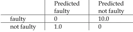
[image:7.595.187.407.539.592.2]As an example, consider a problem that requires classification of items as faulty or not faulty. A typical cost might be as presented in Table 1 which states that if an example is not faulty and is misclassified as faulty the cost would be 1.0 however if an example is faulty and is misclassified as not faulty, the cost would be much higher at 10.0 because this is a more costly error.
TABLE 1. An example of a cost matrix for a two-class problem
Predicted faulty
Predicted not faulty faulty 0 10.0 not faulty 1.0 0
Suppose, now that we use a data mining algorithm to learn a model to classify whether an item is faulty or not, and when evaluated, the model is known to incorrectly classify faulty items 20% of time, and classifies items that are not faulty as faulty at a rate of 30%. Suppose also that the model utilises two attributes, a1 and a2 in 30% and 80% of the cases respectively,
7 Table 1, and the cost of attributes, the expected cost is the sum of the expected cost due to misclassification and the expected cost of classification:
[0.2*10 + 0.3*1] + [0.3*2 + 0.8*1] = 3.7
More formally, given a cost matrix for an n class problem with m attributes, where: Ci,j
represent the cost of classifying an example of class i as class j, Pi,j represents the probability
of classifying an example of class i as j, Pak and Cak represent the probability and cost of the
kth attribute , the expected cost is defined by:
In general, the aim is to develop algorithms that learn classifiers that minimize this expected cost of misclassification as well as the cost of gaining the information needed to perform the classification[9].
Questions which have arisen in developing suitable algorithms include how can these costs be introduced into the decision tree learning process and at what stage of the process is it better to do this? It is possible to incorporate these costs at any stage of the decision tree induction described earlier but what would be the overall effect of including costs, and what impact could this have on the accuracy rate?
2.2 Game Theory
Game theory is a discipline which deals in trade-off when there may be more than one decision-maker [28, 29].The decision makers, referred to as players, choose a strategy (make a decision) and as a result a reward or pay-off occurs.
8 a single problem, for example a shop keeper reducing prices of his stock in response to a competitor doing likewise, are all situations for which game theory can be applied.
In game theory, decisions are linked to goals and the aim is to use the best strategy in order to reach a goal. Pay-off functions are assigned to strategies in order to help make the decisions. Picking strategies which maximizes pay-off is the desired outcome with a trend towards simplicity; finding the simplest assumption needed is the ideal outcome [33]. Pay-offs are shown using a matrix and strategies can be illustrated using decision-tree like structures. Models are not either right or wrong but useful or not depending on the purpose for which they are used. The models are examined in order to analyse their implications, to either confirm an idea or suggest it is wrong. This analysis should help understand why it is wrong. Each player chooses their actions “simultaneously” in that no player is informed when an action is chosen or what action another player has chosen [29]. The assumption is that actions are chosen once and for all and it is assumed that all players will try to do their best.
Studies by [29, 32, 39] give detailed information about of the main categories of games along with many examples.
9 allocation of money to different projects where the outcome is not known [41, 42, 43, 44, 45, 46, 47, 48, 49, 50]. In these applications trade-off occurs in order that total cost of sending a set of packets on selected routes would not be larger than sending the packets all together on a single route or the trade-off between potential research projects which may prove profitable but this information is only obtained over time. More formally, the aim for these types of bandit problems is to maximize the sum of the rewards in a sequence of T lever pulls, with rewards Ri [40, 42, 51]:
10
3 COST-SENSITIVE DECISION TREE LEARNING USING PRINCIPLES FROM
THE MULTI-ARMED BANDIT PROBLEM
This section develops the algorithm for cost-sensitive decision tree induction which uses the principles of the multi-armed bandit algorithm.
A key step in decision tree learning is the selection of the attribute upon which to split the data. Once an attribute is selected, the data is sub-divided according to the values of the attribute and the process repeated recursively on the subsets until some stopping condition is reached. For algorithms that aim to maximize accuracy, the selection criteria is typically an information theoretic measure, such as information gain, and the stopping criteria can be based on the proportion of examples being in one class. For algorithms that aim to minimize misclassification costs, the selection and stopping condition utilize expected cost, either directly or in combination with an information theoretic measure [11]. When test costs (the costs of gaining the information) are involved, the issue of trade-off between the cost of an attribute and its benefit in minimizing misclassification cost arises. Exploration can determine which combination of attributes minimizes misclassification costs but also minimizes the test costs.
To utilize the multi-arm bandit approach, we view the selection of an attribute during the tree construction process as equivalent to that of selecting a bandit. In principle, any of the strategies outlined in Section 2 could be adopted, though in this paper, we adopt the simplest that meets our needs, namely the ε-first strategy in which all the exploration is done in the first P rounds, and followed by exploitation.
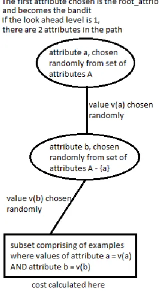
FIGURE 1 illustrates what happens when one bandit that is, an attribute, (i.e, the root
attribute) is selected at random and its lever is pulled. Given a set of attributes A, an attribute a is chosen at random. A value v belonging to attribute a is chosen at random followed by
11
FIGURE 1. Illustration of a single lever pull look-ahead path in the algorithm
Such a lever pull results in a subset containing examples where attribute a equals value v etc. and for which a cost can be calculated, which is the sum of the misclassification costs plus costs associated with the attributes used. In theory, this could result in no examples meeting these criteria. In this case, the particular lever pull would be ignored with no cost being calculated.2
12
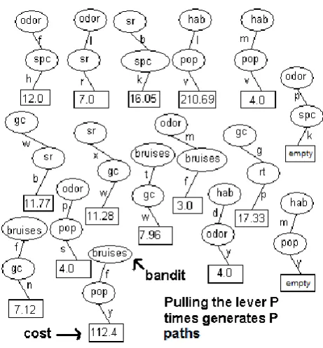
FIGURE 2. Generate P paths and calculate cost at the end of each path
[image:13.595.189.410.600.685.2]FIGURE 2 illustrates P paths which have been generated and the cost calculated at the end of each path as defined in Section 2.1 or marked as empty in cases when there are no examples with the combination of attributes and values specified in a path. In the illustration there are five different attributes chosen; odor, sr, hab, gc and bruises. For each time they have been randomly selected, an attribute value has been chosen.
TABLE 2. Multi-Armed Cost Sensitive Decision Tree (MA-CSDT) algorithm choosing an attribute
attribute summed up cost mean of costs
odor 26.0 6.5
sr 27.33 13.665
hab 218.69 72.89
gc 29.1 14.55
bruises 127.48 42.49
13 with the lowest mean cost is selected. This strategy of first carrying out the lever pulls,
computing the mean and then selecting the bandit is called the ε-first strategy [52]. Bubeck et al. [52] presents a theoretical analysis of this type of bandit strategy showing that the level of simple regret, which is defined as the difference between the optimal and actual reward, decreases exponentially with the number of lever pulls, and that the expected simple regret
) (rp
E can be bounded for a problem with N bandits as the number of lever pulls, P, for each
arm increases (corollary 3 from Bubeck et al.[52]):
P N N r E p ln 2 2 ) (
The probably approximately correct (PAC) framework provides an alternative analysis of the ε-first bandit strategy. In the PAC framework, we are interested in the extent to which it is possible to select an attribute that results in a reward that is within an ε distance of the reward from a best attribute and to do this with a probability of at least 1- . Even-Dar et al.[64] show that the ε-first strategy is PAC learnable by selecting the following number of lever pulls, P, for each of the N arm:3
N P 42 ln 2
Although such results are useful in showing asymptotic convergence, Kuleshov and Precup [66] show that they do not necessarily reflect the performance of the different bandit
strategies in applications. Indeed, a study by Vermorel and Mohri [49] suggests that bandit strategies with the “ best asymptotic guarantees do not provide the better results, and could not have been inferred from a simple comparison of the theoretical results known so far” but also conclude that “the ranking of the strategies changes significantly when switching to real world data”. Perhaps surprisingly, empirical evaluations suggest that the simpler strategies can sometimes outperform the more sophisticated strategies [49, 66]. Thus selecting the
14 number of lever pulls for particular bandit problems, including the one addressed in this paper requires experimentation. Section 4 will describe the approach we use in deciding the number of lever pulls when carrying out an empirical evaluation.
FIGURE 3 presents the top level of the algorithm MA_CSDT illustrated above, where the function exploreAttributes uses the function leverPulls to explore the
combinations of attributes by generating the paths and returning the best attribute to exploit that will trade-off the cost of an attribute against the misclassification cost. The functions
exploreAttributes and leverPulls are defined in FIGURE 4.
MA_CSDT(A, Examples, P, K)
Inputs: A is the set of available attributes Examples are the training examples P is number of lever pulls
K is depth to look ahead Output: DT, a decision tree
if A is empty OR
Proportion of Examples is less than user specified percentage OR
Proportion of examples in the majority class exceeds a threshold return DT as a leaf
class set as the majority class,
except in cases of equal class distribution when it is set to the class which minimizes cost
else
a_exploit = exploreAttributes(A, Examples, P, K)
cost_reduction = misclassification cost without a_exploit – misclassification cost with a_exploit
if cost_reduction > cost of using test a_exploit subset = Split_Data(Examples, a_exploit)
For each subset i
subTreei = MA_CSDT(A – {a_exploit},subseti, P, K) End For
return a DT with test a_exploit and subtrees subTreei
else
return DT as a leaf
class set as the majority class,
except in cases of equal class distribution when it is set to the class which minimizes cost
End
15
FIGURE 4. Definition of exploreAttributes and leverPull
Several authors have observed that when an attribute is recommended using cost, it can lead to a node where the cost of the attribute exceeds the savings [34, 57]; hence a further check is needed to ensure that an attribute is worth exploring before continuing the tree induction process recursively. The stopping condition is similar to that adopted in most tree induction algorithms (such as J48): stopping when the available data is below a user-specified
exploreAttributes(A, Examples, P, K) Inputs: A is the set of attributes
Examples are the training examples P is number of lever pulls
K is depth to look ahead
Output: Attribute, the recommended attribute
/* Rai denotes the cumulative cost of utilizing attribute ai
Nai denotes number of times that attribute ai is chosen as root of path, mean_ai denotes the mean cost for attribute ai
*/
Initialize Rai, Nai, mean_ai to zero for all ai set of attributes A
For j = 1 to P
ai set of attributes A
(Path_ai,Exs) = leverPull(ai,A,K,Examples)
If |Exs|/|Examples| > user specified minimum threshold Rai += cost for ai (Path_ai,Exs)
Nai = Nai + 1
End For
Compute mean_ai = Rai/ Nai for all ai set of attributes A return aj set of attributes A that has the lowest mean_aj cost
End
leverPull(ai, A, K, Es)
Inputs: ai is attribute chosen at random
A is the set of attributes K is depth to look ahead Es is the set of examples
Output: (Path, set of examples)
Select v values of attribute ai
Es_ai = {e Es | attribute ai of example e has value v}
If K=0 then return ([ai], Es_ai)
else begin
aj A-{ai}
(PathAj,Es_aj) = leverPull(aj,A-{ai},K-1, Es_ai)
Path = sequence with ai first followed by PathAj
return (Path, Es_aj)
16 proportion, there are no attributes left, or the proportion of examples in the majority class exceeds a user-specified value. .
The merits of this algorithm are evaluated empirically in the next section.
4 EMPIRICAL COMPARISON
This section presents an empirical evaluation and comparison of MA_CSDT with five other cost-sensitive tree induction algorithms. Our choice of comparison algorithms is based on selecting representative algorithms from the categories of cost-sensitive algorithms identified in [11, 56], which classifies algorithms by the way in which costs are introduced. The
algorithms selected aim to cover five of the most common classes:
Use of costs during construction: The algorithm chosen is EG2 [15] and has been implemented by adapting the J48 algorithm in WEKA.
Bagging: The algorithm chosen is MetaCost [19],which is included in the WEKA package.
Boosting: AdaCostM1 [20] is an adaptation of the algorithm AdaBoostM1 [59] which is included in the WEKA package. The adaptations developed by [20] for the
algorithm AdaCost, have been added to AdaBoostM1 in order that the algorithm AdaCost can process multi-class datasets and be included in the evaluation.
GA methods: ICET has been previously implemented and has been tested by comparing experiments in [8] in order to check the implementation [60].
Stochastic approach: The algorithm chosen is ACT which was implemented and has been tested by repeating and comparison with results in [56].
17 The experimental evaluation was carried out using 15 datasets obtained from the Machine Learning Repository [61]. A range of misclassification costs were used in order to examine the trade-off between the two types of cost used; test costs (the costs associated with
attributes) and misclassification costs. For example misclassification costs were assigned to the classes in a dataset to be higher than the test costs, lower than the test costs and a mixture of high and low values in relation to the test costs. Test costs have either been devised by experts or have been used in other studies [8, 12, 56]. The Appendix shows the ranges of test costs which the dataset contains. Each attribute has been assigned a test cost which is within this range and remains consistent throughout the experiments when that attribute is used. The cost to classify is calculated and normalized as per Turney’s method described in [8]. The other parameter we need to set is the number of lever pulls. As described in Section 3,
although there are theoretical bounds that could be used to set the number of lever pulls, these are not sufficiently tight, and several studies have suggested that the optimal value is problem dependent [49,66]. In these empirical evaluations, we use the maximum number of possible paths, which are computed from the number of attributes and their possible values, as a guide to setting the number of lever pulls in advance. The Appendix provides details of the data sets, cost matrices and number of lever pulls used in these experiments.
The methodology utilized included randomly creating 10 training and testing pairs consisting of 70% of the dataset for training with the remaining used for testing.
18 In applications, the ideal is, of course, that we are able to maximize accuracy and minimize costs. However, this is not always possible and as mentioned earlier, there is often a trade-off between accuracy and costs. Thus, there is a need to consider situations in which a user may wish to optimize costs, in which case one can select the trees that minimize cost, or
alternatively there may be a preference for more accurate trees. Hence, the empirical evaluation in Section 4.1 presents results from these two strategies.
4.1 Empirical results
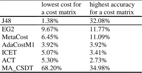
TABLE 3 presents the percentage of time that each cost-sensitive algorithm achieved the lowest costs and the highest accuracy.
[image:19.595.183.415.471.590.2]The costs for each dataset returned by each algorithm have been averaged over all the cost matrices. Cases where no tree is produced are excluded from consideration with regard to their performance.
TABLE 3. Percent that each cost-sensitive algorithm achieves the lowest cost or highest accuracy for a cost
matrix
lowest cost for a cost matrix
highest accuracy for a cost matrix
J48 1.38% 32.08%
EG2 9.67% 11.77%
MetaCost 6.45% 11.09%
AdaCostM1 3.92% 3.92%
ICET 5.07% 3.41%
ACT 5.30% 2.73%
MA_CSDT 68.20% 34.98%
19 The “cost-based” strategy results in the lowest cost on the datasets diabetes, flare, heart, hepatitis, iris, mushroom, nursery, tic-tac-toe and wine. However in most cases, this results in a large sacrifice of the accuracy rate obtained.
20
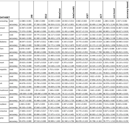
TABLE 4. Results from all datasets for each of the algorithms
J48 EG
2 M e ta C o s t A d a C o s tM 1 IC E T
ACT cost
-b ased a c c u ra c y -b a s e d
annealing cost 12.080 ± 0.001 1.080 ± 0.000 12.093 ± 0.003 10.933 ± 0.012 2.060 ± 0.002 2.747 ± 0.004 1.280 ± 0.001 2.027 ± 0.002
accuracy 97.340 ± 0.000 97.260 ± 0.000 96.924 ± 0.212 95.267 ± 0.851 95.140 ± 0.635 83.499 ± 1.544 86.747 ± 3.243 95.758 ± 0.063 breast cost 32.967 ± 0.039 26.540 ± 0.062 1.887 ± 0.017 1.787 ± 0.016 18.007 ± 0.066 19.260 ± 0.047 26.460 ± 0.016 31.867 ± 0.026
accuracy 72.370 ± 0.000 66.660 ± 0.000 51.433 ± 4.830 51.491 ± 4.846 68.527 ± 0.154 56.022 ± 4.068 60.805 ± 2.238 68.627 ± 0.819 car cost 47.883 ± 0.019 39.775 ± 0.014 46.117 ± 0.025 40.850 ± 0.047 11.117 ± 0.035 11.542 ± 0.025 19.192 ± 0.027 32.775 ± 0.035
accuracy 90.640 ± 0.000 81.900 ± 0.000 86.493 ± 1.076 80.383 ± 3.340 71.267 ± 1.248 58.968 ± 5.181 57.080 ± 5.108 71.826 ± 0.544 diabetes cost 38.047 ± 0.015 33.907 ± 0.012 4.980 ± 0.032 4.193 ± 0.029 19.773 ± 0.033 12.640 ± 0.019 12.280 ± 0.030 30.940 ± 0.023
accuracy 75.880 ± 0.000 76.090 ± 0.000 52.771 ± 3.898 52.732 ± 3.873 70.207 ± 0.970 61.171 ± 2.120 62.810 ± 1.858 76.054 ± 0.176 flare cost 8.678 ± 0.007 2.089 ± 0.008 9.678 ± 0.017 14.067 ± 0.036 3.289 ± 0.007 3.422 ± 0.008 3.667 ± 0.008 6.267 ± 0.013
accuracy 89.440 ± 0.000 89.440 ± 0.000 76.504 ± 9.293 81.210 ± 4.111 89.033 ± 0.052 79.026 ± 7.789 84.838 ± 2.781 89.452 ± 0.051 glass cost 35.783 ± 0.019 24.050 ± 0.011 32.483 ± 0.023 31.050 ± 0.024 22.500 ± 0.014 15.444 ± 0.023 16.711 ± 0.019 34.250 ± 0.019
accuracy 68.060 ± 0.000 70.730 ± 0.000 57.852 ± 2.196 55.587 ± 2.569 63.944 ± 0.749 37.594 ± 1.116 44.954 ± 3.319 71.971 ± 0.184 heart cost 29.633 ± 0.008 13.027 ± 0.019 5.187 ± 0.027 4.373 ± 0.024 16.973 ± 0.017 10.253 ± 0.023 5.333 ± 0.002 10.133 ± 0.012
accuracy 75.750 ± 0.000 75.670 ± 0.000 53.528 ± 2.235 53.461 ± 2.189 74.820 ± 0.337 63.525 ± 1.676 65.545 ± 0.815 76.957 ± 0.167 hepatitis cost 28.240 ± 0.006 25.027 ± 0.034 4.753 ± 0.024 4.500 ± 0.024 21.107 ± 0.027 19.193 ± 0.021 6.027 ± 0.012 18.327 ± 0.019
accuracy 87.350 ± 0.000 83.970 ± 0.000 56.499 ± 8.104 57.622 ± 7.629 86.260 ± 0.484 78.069 ± 2.141 70.822 ± 3.826 87.252 ± 0.470 iris cost 33.333 ± 0.019 29.267 ± 0.013 34.211 ± 0.023 34.244 ± 0.027 21.867 ± 0.010 9.822 ± 0.035 6.356 ± 0.025 33.389 ± 0.026
accuracy 93.660 ± 0.000 90.020 ± 0.000 92.309 ± 1.627 92.046 ± 1.638 78.500 ± 2.167 57.856 ± 8.911 46.723 ± 6.331 94.688 ± 0.111 krk cost 44.678 ± 0.012 41.756 ± 0.020 43.744 ± 0.013 41.928 ± 0.013 31.244 ± 0.035 40.189 ± 0.016 34.978 ± 0.022 43.483 ± 0.017
accuracy 53.560 ± 0.000 33.800 ± 0.000 49.859 ± 0.700 49.036 ± 0.910 25.950 ± 2.503 22.237 ± 1.075 16.077 ± 0.623 30.029 ± 0.312 mushroomcost 2.341 ± 0.005 1.351 ± 0.003 2.348 ± 0.005 1.539 ± 0.005 1.708 ± 0.004 2.641 ± 0.005 1.300 ± 0.002 1.658 ± 0.002
accuracy 100.000 ± 0.000 100.000 ± 0.000 99.748 ± 0.199 79.111 ± 6.252 99.607 ± 0.082 96.171 ± 3.089 98.551 ± 0.028 98.585 ± 0.025 nursery cost 34.793 ± 0.040 35.367 ± 0.040 33.947 ± 0.041 33.042 ± 0.041 16.685 ± 0.028 18.973 ± 0.036 16.382 ± 0.030 22.496 ± 0.026
accuracy 96.237 ± 0.000 95.498 ± 0.000 91.567 ± 1.349 87.258 ± 2.729 66.880 ± 5.790 59.397 ± 6.644 48.663 ± 4.867 70.393 ± 3.697 soybean cost 6.460 ± 0.003 6.827 ± 0.003 6.193 ± 0.003 6.287 ± 0.004 6.553 ± 0.003 14.573 ± 0.006 7.513 ± 0.004 8.020 ± 0.004
accuracy 90.330 ± 0.000 87.660 ± 0.000 87.421 ± 0.946 82.641 ± 0.924 88.267 ± 0.187 80.369 ± 0.453 83.594 ± 1.301 87.605 ± 0.181 tictactoe cost 27.840 ± 0.017 27.820 ± 0.017 7.767 ± 0.031 4.827 ± 0.028 16.773 ± 0.021 11.907 ± 0.018 9.027 ± 0.028 19.720 ± 0.031
accuracy 83.670 ± 0.000 83.890 ± 0.000 57.475 ± 4.311 54.195 ± 4.401 74.767 ± 1.978 80.003 ± 2.236 61.333 ± 3.043 75.170 ± 0.338 wine cost 18.256 ± 0.002 13.022 ± 0.002 16.822 ± 0.004 15.211 ± 0.012 12.867 ± 0.004 5.044 ± 0.017 10.600 ± 0.001 17.822 ± 0.004
accuracy 93.470 ± 0.000 87.510 ± 0.000 90.909 ± 1.693 81.560 ± 4.796 86.478 ± 0.329 45.798 ± 4.363 78.777 ± 1.522 93.456 ± 0.259
DATASET
The algorithm MA_CSDT does not perform well on the datasets car, nursery and krk. No algorithm returns a higher accuracy rate than J48 on these datasets, although it accomplishes this at a greater cost than each of the other algorithms including both strategies of MA_CSDT. MetaCost and AdaCostM1 get closer to the accuracy rate of J48 than any other algorithm and
21 MetaCost and AdaCostM1 also perform better on datasets soybean and wine than other
cost-sensitive algorithms. ICET does not perform as well as J48 on the soybean dataset but for all other datasets, it does obtain a lower cost than J48, but also has problems with car, iris, nursery, tic-tac-toe and wine. Along with all other algorithms, ICET also encountered problems whilst processing the krk dataset.
4.2 Discussion of the outcome of the empirical evaluation
As TABLE 3 summarizes, the MA_CSDT algorithm returns the lowest cost for a cost matrix 68.2% of the time and the highest accuracy for a cost matrix 34.98% of the time. Each time the highest accuracy is achieved, its corresponding cost is lower than that of J48. The main aim, to achieve the same or higher rate of accuracy more cost-effectively than the accuracy-based algorithm J48 has been met for the datasets annealing, flare, glass, iris, heart and mushroom.
For the datasets breast, diabetes, hepatitis, tic-tac-toe and wine a sacrifice of less than between 1% to 3% of the accuracy rate returned by J48 results in a lower cost. For the remaining datasets, car, krk, nursery and soybean, this aim has not been met.
By looking at the two strategies “cost-based” and “accuracy-based” it is apparent that a trade-off is required. The heart dataset is representative of the datasets on which MA_CSDT produces a high accuracy rate in a more cost-effective way. Almost all such cases are a result of adopting the “accuracy-based” strategy. In contrast, although the “cost-based” strategy can results in lower cost, the corresponding accuracy rates are always lower than the J48
algorithm.
The krk dataset is representative of poor results, where the MA_CSDT algorithm has been unable to minimize cost as well as retain accuracy. The accuracy-based algorithm J48 achieved the highest accuracy overall, with only two of the cost-sensitive algorithms
22 rate with a small reduction in costs. EG2, ICET and ACT also failed to achieve a comparable accuracy rate but do manage to at least reduce costs.
On examination of the trees induced, the most likely cause of this is that the MA_CSDT algorithm either grows trees that are too small in comparison with the size of the dataset, which has a large number of examples in the training set, or grows a tree which is far too large with over 20,000 leaves. The paths in these trees are comprised of 6 attributes in order to reach the leaves. The smaller trees have paths to the leaves which consist of two or three attributes. The conclusion reached is that the large number of examples contributes to the problems of processing this dataset. In each training file there are approximately 20,000 examples. Pruning or stopping the tree build early results in many examples at the leaf nodes which results in low accuracy. Allowing the tree to grow fully results in overgrown trees with few examples at the node, which results in higher test costs but still does not improve
accuracy. The ACT algorithm also produces trees which follow this pattern of either too small or too large and is also not very successful on this dataset.
The three algorithms, which produce the better results for this dataset (J48, MetaCost,
AdaCostM1), all produce the same tree which has 3948 leaves. They all choose the same root;
23 This dataset demonstrates that higher accuracy does not always mean lower costs, if to
achieve this, the tree grows uncontrollably. However spending less on test costs does not always work either as money saved on tests may be spent on misclassification costs.
In some cases either pruning a tree results in no tree being left or that no tree has been grown in the first instance; for MetaCost and AdaCostM1 the reason that no trees have been
produced on some occasions, is that the process stops as all the examples belong to one class. In the case of AdaCostM1 this will be owing to the initial weight procedure and in the case of MetaCost, owing to the way that this algorithm re-labels the training example with the class
that minimizes the cost, as described in Section 5.2.2 in [11].
In the case of the flare dataset, each of the other algorithms fails to grow trees for some of the cost matrices. In particular EG2 does not grow any trees at all, ICET does not grow trees 84% of the time and even J48 does not grow any trees 70% of the time. After careful examination of the output, it has been concluded that the lack of trees are as a result of the class
distribution of the dataset which causes the majority of trees to be pruned back to nothing. The majority class in the whole dataset has 88.9% of the examples in it. Pruning techniques would most likely determine that sub-trees were not able to improve on the results of the original dataset and so would be converted into leaves, resulting in a large percentage of no models being produced.
24
5 CONCLUSIONS AND FUTURE WORK
This paper has developed a new algorithm, MA_CSDT, for cost-sensitive decision tree induction based on the principles and concept of the multi-armed bandit problem. An empirical evaluation and comparison of the algorithm with six representative cost-sensitive algorithms on 15 data sets shows promising results, with MA-CSDT producing lowest cost trees in 68% of the trials. The algorithm has helped explore and confirm a research hypothesis, that cost-sensitive learning involves a trade-off between the decisions based on accuracy and decisions based on cost and that there is merit in utilizing multi-arm bandits for this problem.
By using a framework which explores strategies based on cost, a compromise between these viewpoints can be reached in the majority of cost-sensitive problems. The nature of the domain dictates the importance of this aim. Whilst some domains may err on the side of caution and prefer to sacrifice the accuracy rate rather than incur high misclassification costs, there are many domains where this is not acceptable. In these domains, if a classifier can be found which will minimize costs, but at the same time be as accurate as an accuracy-based classifier, this is more desirable.
Although many different approaches have been attempted for inducing cost-sensitive trees [11], this is a first attempt at using the concepts of multi-arm bandits for this problem, and there is significant potential for future work. First, on the theoretical front, it is worth
25 successive rounds of resampling, leading to tighter bounds and which could result in further improvements. For larger data sets, where computational cost is a major issue, more sophisticated strategies such as Gaussian Processes Bandits [45, 48, 49], could be also be attempted to optimise the number of lever pulls in cost-sensitive decision tree learning.
ACKNOWLEDGEMENTS
The authors would like to thank the reviewers whose comments have led to improvements in the paper, especially in encouraging the authors to include the relationship with the PAC learnability results presented in Section 3.
REFERENCES
[1] Quinlan, J. R. (1986). Induction of decision trees. Machine Learning 1, Kluwer Academic Publishers, Boston, 81-106.
[2] Quinlan, J. R. (1979). Discovering rules by induction from large collections of examples. In Expert Systems in the Micro Electronic Age, D. Michie, Ed., Edinburgh University Press, 168–201.
[3] Quinlan, J. R. (1983). Learning efficient classification procedures and their application to chess end games. In Machine Learning: An Artificial Intelligence Approach, Michalski, Garbonell and Mitchell Eds., Tioga Publishing Company, Palo Alto, CA.
[4] Quinlan, J. R. (1993). C4.5: Programs for machine learning. Morgan Kaufman, San Mateo, CA.
26 [6] Murthy, S., Kasif, S. and Salzberg, S. (1994). A System for induction of oblique decision trees. Journal of Artificial Intelligence Research, 2, 1-32.
[7] Elkan, C. (2001). The foundations of cost-sensitive learning. In Proceedings of 17th International Joint Conference on Artificial Intelligence (IJCAI’01), Morgan Kaufmann, San Francisco, USA, Vol. 2, 973 – 978.
[8] Turney, P. D. (1995). Cost-sensitive classification: empirical evaluation of a hybrid genetic decision tree induction algorithm. Journal of Artificial Intelligence Research, 2, 369-409.
[9] Turney, P. D. (2000). Types of cost in inductive concept learning. Workshop on Cost-Sensitive Learning at the 17th International Conference on Machine Learning (WCSL at ICML-2000), Stanford University, California, 15-21.
[10] Quinlan, J. R., Compton, P. J., Horn, K. A. and Lazarus, L. (1987). Inductive knowledge acquisition: a case study. Applications of expert systems, Chapter 9, J Ross Quinlan (Ed), Based on the proceedings of the second Australian Conference. Turing Institute Press with Addison-Wesley Publishing Co. ISBN 0-201-17449-9, 137-156.
[11] Lomax, S. and Vadera, S. (2013). A survey of cost-sensitive decision tree induction algorithms. ACM Computing Surveys, Vol. 45, No. 2, Article 16.
http://doi.acm.org/10.1145/2431211.2431215
[12] Lomax, S. and Vadera, S. (2011). An empirical comparison of cost-sensitive decision tree induction algorithms. Expert Systems The Journal of Knowledge Engineering, July, Vol. 28, No 3, 227 – 268.
27 [14] Ting, K. (2000). An empirical study of MetaCost using boosting algorithms. In
Proceedings of the 11th European Conference on Machine Learning. Lecture Notes in Computer Science, vol. (1810), Springer, 413–425.
[15] Núnez. (1991). The use of background knowledge in decision tree induction. Machine Learning 6, Kluwer Academic Publishers, Boston, 231-250.
[16] Tan, M. (1993). Cost-sensitive learning of classification knowledge and its applications in robotics. Machine Learning, 13, 7–33.
[17] Tan, M. and Schlimmer J. (1989). Cost-Sensitive concept learning of sensor use in approach and recognition. In Proceedings of the 6th International Workshop on Machine Learning (ML ’89).392–395.
[18] Norton, S.W. (1989). Generating better decision trees. In Proceedings of the 11th International Joint Conference on Artificial Intelligence (IJCAI ’89), 800–805.
[19] Domingos, P. (1999). MetaCost: A general method for making classifiers cost-sensitive. In Proceedings of the fifth ACM SIGKDD international conference on Knowledge discovery and data mining. ACM New York, NY, USA, 155–164.
[20] Fan, W., Stolfo, S. J., Zhang, J. and Chan, P. K. (1999). AdaCost: misclassification cost-sensitive boosting. 16th International Conference on Machine Learning, June 27-30 1999, Bled, Slovenia, 97-105.
[21] Merler, S., Furlanello, C., Larcher, B. and Sboner, A. (2003). Automatic model selection in cost-sensitive boosting. Inf. Fusion 4, 1, 3–10.
[22] Esmeir, S. and Markovitch, S. (2004). Lookahead-based algorithms for anytime
28 [23] King, R. D., Feng, C. and Sutherland, A. (1995). STATLOG: Comparison of
classification algorithms on large real-world problems. Applied Artificial Intelligence, 01/1995, 9, 289 – 333.
[24] Abdelmessih, S.D., Shafait, F., Reif, M. and Goldstein, M. (2010). Landmarking for meta-learning using RapidMiner. In German Research Center for Artificial Intelligence, Germany, viewed on-line on 24.1.14 at http://www.mendeley.com/research/landmarking-metalearning-using-rapidminer
[25] Bensusan, H. and Giraud-Carrier, C. (2000). Discovering task neighbourhoods through landmark learning performances. In Lecture Notes in Computer Science, Vol 1910, Principles of Data Mining and Knowledge Discovery, Springer Berlin Heidelberg, 325 – 330.
[26] Shilbayeh, S. A. and Vadera, S., Feature selection in meta learning framework,
Proceedings of the Science and Information Conference, London, To appear in August 2014. [27] Cesa-Bianchi, N. and Lugosi, G. (2006). Prediction, learning and games. Cambridge University Press, New York.
[28] Davis, M. D. (1983). Game theory a nontechnical introduction. Dover Publications Inc, Mineola, NY, USA.
[29] Osborne. M. J., 2004). An introduction to game theory. Oxford University Press, New York, USA.
[30] Nash, J. F. (1950a). Equilibrium points in N-person games. Proceedings of the National Academy of Sciences of the United States of America, 36, 48 – 49.
[31] Nash, J. F. (1950b). Non-cooperative games. Doctoral dissertation, Princeton University, reprinted in The Essential John Nash (Harold W Kuhn and Sylvia Nasar, Eds), 53 – 84). Princeton University Press 2002.
29 [33] Rasmusen, E. (2001). Games and information an introduction to game theory. Third Edition, Blackwell Publishers Ltd, Oxford, UK.
[34] Ling, C. X., Yang, Q., Wang, J. and Zhang, S. (2004). Decision trees with minimal costs. ACM International Conference Proceeding Series 21st international conference on Machine learning, Banff, Alberta, Canada, Article No. 69, ISBN: 1-58113-828-5. ACM Press New York, NY, USA.
[35] Ting, K. and Zheng, Z. (1998a). Boosting cost-sensitive trees. Proceedings of 1st
International Conference on Discovery Science, Springer-Verlag, London, LNCS, 1532, 244– 255.
[36] Ting, K. M. and Zheng, Z. (1998b). Boosting trees for cost-sensitive classifications. In Machine Learning: ECML-98 10th European Conference on Machine Learning, Chemnitz, Germany. Springer, 190-195.
[37] Zadrozny, B., Langford, J. and Abe, N. (2003a). A simple method for cost-sensitive learning. Technical Report RC22666, IBM, 2003.
http://citeseer.ist.psu.edu/viewdoc/summary?doi=10.1.1.7.7947
[38] Zadrozny, B., Langford, J. and Abe, N. (2003b). Cost-sensitive learning by cost-proportionate example weighting. Third IEEE International Conference on Data Mining, November 19 - 22, 2003, Melbourne, Florida, USA, 435.
[39] Binmore, K. (2007). Game theory a very short introduction. Oxford University Press Inc, New York.
[40] Robbins, H. (1952). Some aspects of the sequential design of experiments. Bulletin American Mathematical Society, 55, 527–535.
30 [42] Auer, P., Cesa-Bianchi, N. and Fischer, P. (2002). Finite-time analysis of the multi-armed bandit problem. Machine Learning 47, 235-256.
[43] Auer, P., Cesa-Bianchi, N., Freud, Y. and Schapire, R.E. (1995). Gambling in a rigged casino: the adversarial multi-armed bandit problem. Internal Report 223-98, DSI, Università di Milano, Italy, Foundations of Computer Science, Proceedings of 36th Annual Symposium, October 23-25, Milwaukee, USA, 322 – 331.
[44] Berry, D. A. and Fristedt, B. (1985). Bandit problems: sequential allocation of experiments. Monographs on Statistics and Applied Probability, London: Chapman & Hall, ISBN 0-412-24810-7.
[45] Dorard, L., and Shawe-Taylor, J. (2010). Gaussian process bandits for tree search. University College London, available on-line at
http://ucl.academia.edu/LouisDorard/Papers/273653/Gaussian_Process_Bandits_for_Tree_Se arch. viewed 8/2/2011. 2010
[46] Dorard, L., Glowacka, D. and Shawe-Taylor, J. (2009). Gaussian process modelling of dependencies in multi-armed bandit problems. Proceedings of 10th International Symposium on Operational Research (SOR), September 23-25, Nova Gorica, Slovenia.
[47] Gittins, J. C. (1989). Multi-armed bandit allocation indices. Wiley-Interscience Series in Systems and Optimization, Chichester: John Wiley & Sons, Ltd, ISBN 0-471-92059-2. [48] Grünewälder, S., Audibert, J-Y., Opper, M. and Shawe-Taylor, J. (2010). Regret bounds for Gaussian process bandit problems. Proceedings of the 13th International Conference on Artificial Intelligence and Statistics, Vol. 9 of JMLR, Chia Laguna Resort, Sardinia, Italy. [49] Vermorel, J. and Mohri, M. (2005), Multi-armed bandit algorithms and empirical
31 [50] Auer, P. (2002). Using confidence bounds for exploitation-exploration trade-offs. Journal of Machine Learning Research, 3, 397-422.
[51] Shawe-Taylor, J. 2010. Multivariate bandits and their applications. In Intelligent
Information Processing, IIP, Presentation Slides, 15 October, held at Lowry Centre, Salford. [52] Bubeck, S., Munos R. and Stoltz, G. 2009. Pure exploration in multi-armed bandit problems. Algorithmic Learning, Lecture Notes in Computer Science, Volume 5809, 23-37. [53] Audibert, J. Y., and Bubeck, S. 2010. Best arm identification in multi-armed bandits. In COLT-23th Conference on Learning Theory-2010, Jun 2010, Haifa, Israel, 13 p.
[54] Gabillon, V., Ghavamzadeh, M. and Lazaric, A. 2012. Best Arm Identification: A Unified Approach to Fixed Budget and Fixed Confidence. Advances in Neural Information Processing Systems 25, 3212-3220.
[55] Watkins C. J. C. H. 1989. Learning from Delayed Rewards. Ph.D. thesis. Cambridge University.
[56] Esmeir, S. and Markovitch, S. (2008). Anytime induction of low-cost, low-error
classifiers: a sampling-based approach. Journal of Artificial Intelligence Research 33, 1-31. [57] Lomax, S. (2013). Cost-sensitive decision tree learning using a multi-armed bandit framework. PhD Thesis. University of Salford.
[58] Lomax, S., Vadera, S. and Saraee, M. (2012). A multi-armed bandit approach to cost-sensitive decision tree learning. In Data Mining Workshops (ICDMW), 2012 IEEE 12th International Conference, 10-13 December 2012, Brussels, Belgium,
http://ieeexplore.ieee.org/xpl/login.jsp?tp=&arnumber=6406437&url=http%3A%2F%2Fieeex plore.ieee.org%2Fxpls%2Fabs_all.jsp%3Farnumber%3D6406437 162 - 168.
32 [60] Vadera, S. and Ventura, D. (2001). A comparison of cost-sensitive decision tree learning algorithms. Second European Conference in Intelligent Management Systems in Operations, 3– 4 July, University of Salford, Operational Research Society, Birmingham, UK, 79-86. [61] Bache, K. and Lichman, M. (2013). UCI Machine Learning Repository,
http://archive.ics.uci.edu/ml, Irvine, CA: University of California, School of Information and
Computer Science.
[62] Aodha, O.M. and Brostow, G.J. (2013). Revisiting example dependent cost-sensitive learning with decision trees, in Proc of the IEEE International Conference on Computer Vision, Washington, DC, USA, pp. 193–200.
[63] Bahnsen, A. C., Aouada, D., and Ottersten, B. (2015). Example-dependent cost-sensitive decision trees. To appear in Expert Systems with Applications, doi:
http://dx.doi.org/10.1016/j.eswa.2015.04.042
[64] Even-Dar, E., Mannor, S., and Mansour, Y. (2002). PAC bounds for multi-arm bandits and Markov decision processes, In Fifteenth Annual Conference on Computational Learning Theory (COLT), pp255-270
[65] Fern, A. (n.d). Monte-Carlo Planning: Introduction and Bandit Basics,
http://web.engr.oregonstate.edu/mcai/mc_plan_library/mcp-bandits.pdf, accessed 1/11/15
[66] Kuleshov,A. and Precup, D. (2000). Algorithms for the multi-arm bandit problem, Journal of Machine Learning Research, 1, pp1-48
33
APPENDIX
A1 Dataset Information
dataset name no classes (attributes) test cost range (total test cost) grouped
annealing 5 (24) 50.0 – 2000.0 (15850.0) yes
breast 2 (9) 5.02877 – 93.0188 (368.9732) yes
Car 4 (6) 5.58562 – 98.6441 (258.7396) yes
diabetes 2 (6) 1.00 – 22.78 (44.39) yes
Flare 3 (10) 4.36544 – 96.5457 (382.248) yes
glass 6 (7) 13.3987 – 78.2133 (393.804) yes
heart 2 (11) 1.0 – 102.9 (592.3) yes
hepatitis 2 (16) 1.0 – 8.3 (35.84) yes
Iris 3 (4) 7.65056 – 98.2458 (206.6928) no
Krk 18 (6) 7.11229 – 89.3119 (260.0522) no
mushroom 2 (21) 1.0 – 7.0 (63.0) no
nursery 5 (8) 8.21288 – 98.6441 (185.9273) yes
soybean 15 (35) 5.0 – 10.0 (270.0) yes
tic-tac-toe 2 (9) 1.0 (9.0) no
wine 3 (13) 5.86631 – 98.5054 (697.0051) yes
Full details of the datasets and the costs associated with each attribute are given in [57].
A2 Value of P for each dataset used in the experiments
The Table below lists the values of the number of lever pulls (P) used for each data set. The values of P were allocated for each dataset by calculating the number of potential unique paths there would be in a decision tree given the number of attributes and their values. This was then used as a guideline to allocate values so that there are five values for each dataset. These values are (1) lower than the potential unique path value; (2) rounded down from the potential unique path value; (3) the potential unique path value; (4) higher than the potential unique path value and (5) a much lower value than any of the previous values. The identifiers (6) and (7) were specially included for soybean and used in one smaller experiment. This was done as the soybean dataset has a longer process time than all other datasets.
34
Identification of the value of P for each dataset
depth (k) 1 1 2 3 4 5 6 7
dataset
annealing 7000 8000 8312 10000 1000 breast 1500 2000 2152 5000 500
car 200 300 366 500 50
diabetes 150 180 184 300 30
flare 700 800 898 2000 100
glass 200 300 338 1000 50
heart 500 600 658 1000 100
hepatitis 800 1000 1082 1500 100
iris 75 100 108 500 30
krk 1000 1300 1312 1500 100
mushroom 10000 12000 12624 15000 1000 nursery 500 600 632 1000 100
soybean 1000 3000 9104 5000 50 8000 9000 tic-tac-toe 500 600 648 1000 100
wine 1000 1200 1256 1500 100 depth (k) 2
dataset
car 3000 4000 5082 6000 diabetes 500 1000 1776 3000 glass 3000 4000 4692 6000
iris 500 600 648 1000
A3 Details of the misclassification costs used in all experiments
For the two class datasets, a range of misclassification costs have been chosen which are a mixture of higher and lower values than the test costs in the dataset. This has then been reversed so that each class costs each value in turn during the experiments. This is to remove any advantages with regard to class distribution within each dataset.
2-class datasets
cost matrix
1 2 3 4 5 6 7 8 9 10 11 12 13 14 15
class
1 1 1 1 1 1 1 1 1 10 50 100 500 1000 5000 10000 2 10000 5000 1000 500 100 50 10 1 1 1 1 1 1 1 1
35 3-class datasets
cost matrix 1 2 3 4 5 6 7 8 9
(M) (L) (H)
class
1 1 100 10 1 10 5 150 250 200 2 10 1 100 5 1 10 200 150 250 3 100 10 1 10 5 1 250 200 150
4-class datasets
cost matrix 1 2 3 4 5 6 7 8 9 10 11 12
(M) (L) (H)
class
1 1 500 100 10 1 20 10 5 150 300 250 200 2 10 1 500 100 5 1 20 10 200 150 300 250 3 100 10 1 500 10 5 1 20 250 200 150 300 4 500 100 10 1 20 10 5 1 300 250 200 150
5-class dataset: annealing
cost matrix 1 2 3 4 5 6 7 8 9 10 11 12 13 14 15
(M) (L) (H)
class
1 100 10000 5000 1000 500 150 350 300 250 200 1000 5000 4000 3000 2000 2 500 100 10000 5000 1000 200 150 350 300 250 2000 1000 5000 4000 3000 3 1000 500 100 10000 5000 250 200 150 350 300 3000 2000 1000 5000 4000 4 5000 1000 500 100 10000 300 250 200 150 350 4000 3000 2000 1000 5000 5 10000 5000 1000 500 100 350 300 250 200 150 5000 4000 3000 2000 1000
5-class dataset: nursery
cost matrix 1 2 3 4 5 6 7 8 9 10 11 12 13 14 15
(M) (L) (H)
class
1 1 1000 500 100 10 1 50 20 10 5 150 350 300 250 200 2 10 1 1000 500 100 5 1 50 20 10 200 150 350 300 250 3 100 10 1 1000 500 10 5 1 50 20 250 200 150 350 300 4 500 100 10 1 1000 20 10 5 1 50 300 250 200 150 350 5 1000 500 100 10 1 50 20 10 5 1 350 300 250 200 150
6-class dataset: glass
cost matrix 1 2 3 4 5 6 7 8 9 10 11 12 13 14 15 16 17 18
(M) (L) (H)
class
36
5 500 100 50 10 1 1000 50 20 10 5 1 70 350 300 250 200 150 400 6 1000 500 100 50 10 1 70 50 20 10 5 1 400 350 300 250 200 150
As there are so many classes in the final two datasets, a similar process to the two class datasets was used to allocate misclassification costs. In these cases a range of costs were chosen and allocated to each class (cost matrix 1). Then for each subsequent cost matrix identifier the misclassification costs were moved round one place. The result is that each class is allocated each misclassification cost in turn.
15-class dataset: soybean
cost matrix 1 2 3 4 5 6 7 8 9 10 11 12 13 14 15 class
1 1 700 650 600 550 500 450 400 350 300 250 200 150 100 50 2 50 1 700 650 600 550 500 450 400 350 300 250 200 150 100 3 100 50 1 700 650 600 550 500 450 400 350 300 250 200 150 4 150 100 50 1 700 650 600 550 500 450 400 350 300 250 200 5 200 150 100 50 1 700 650 600 550 500 450 400 350 300 250 6 250 200 150 100 50 1 700 650 600 550 500 450 400 350 300 7 300 250 200 150 100 50 1 700 650 600 550 500 450 400 350 8 350 300 250 200 150 100 50 1 700 650 600 550 500 450 400 9 400 350 300 250 200 150 100 50 1 700 650 600 550 500 450 10 450 400 350 300 250 200 150 100 50 1 700 650 600 550 500 11 500 450 400 350 300 250 200 150 100 50 1 700 650 600 550 12 550 500 450 400 350 300 250 200 150 100 50 1 700 650 600 13 600 550 500 450 400 350 300 250 200 150 100 50 1 700 650 14 650 600 550 500 450 400 350 300 250 200 150 100 50 1 700 15 700 650 600 550 500 450 400 350 300 250 200 150 100 50 1
18-class dataset: krk
cost matrix 1 2 3 4 5 6 7 8 9 10 11 12 13 14 15 16 17 18 class
37