Fractional Fourier Transform Algorithms for Interference Suppression: Rotational Parameter and Mean Square Error Comparison

International Journal of Emerging Technology and Advanced Engineering

Website: www.ijetae.com (ISSN 2250-2459, ISO 9001:2008 Certified Journal, Volume 6, Issue 10, October 2016)

46

Fractional Fourier Transform Algorithms for Interference

Suppression: Rotational Parameter and Mean Square Error

Comparison

Seema Sud

The Aerospace Corporation, 4851 Stonecroft Blvd. Chantilly, VA 20151

Abstract— Minimum mean-square error (MMSE) filtering in the Fractional Fourier Transform (FrFT) domain, or MMSE-FrFT, performs better interference suppression (IS) over the fast Fourier Transform (FFT) when the signal-of-interest (SOI) or interference is non-stationary. This technique estimates the optimum FrFT rotational parameter, ‘a’, as that which gives the MMSE between a signal and its estimate. However, MMSE filtering requires computational covariance matrix inversion. Furthermore, few samples must be used to form the covariance matrix in non-stationary environments, where statistics rapidly change, but MMSE techniques usually require many samples. Hence, MMSE-FrFT filtering results in errors. In this paper, we describe three recently developed algorithms for FrFT domain IS that each estimate ‘a’ differently: (1) using domain decomposition (DD), (2) using the relation of the FrFT to the Wigner Distribution (WD), and (3) using the correlations subtraction architecture of the multistage Wiener filter (CSA-MWF). The former two algorithms then use MMSE to perform the filtering, whereas the last uses the CSA-MWF. We compare the proposed algorithm to the MMSE-FrFT algorithm by simulation, and we show that all three new algorithms outperform MMSE-FrFT by up to several orders of magnitude, using just N = 4 samples per block. The CSA-MWF is the most robust in low Eb/N0, e.g. Eb/N0 < 5 dB. At high Eb/N0, the MMSE, DD and WD algorithms slightly outperform CSA-MWF at low carrier-to interference ratios (CIRs), and all four algorithms perform equally at high CIRs, as expected.

Keywords—Domain Decomposition, Fractional Fourier Transform, MMSE, Multistage Wiener Filter, Wigner Distribution.

I. INTRODUCTION

The Fractional Fourier Transform (FrFT) has numerous applications in fields such as signal and image processing, optics, and quantum mechanics ([7] and [8]). It is a powerful tool for separating a signal-of-interest (SOI) from interference and/or noise when the statistics of either are non-stationary, as is often the case [10].

The FrFT translates the received signal to an axis in the time-frequency plane, known as the Wigner Distribution (WD), where the SOI and interference may be separable, when they are not separable in the time domain or in the frequency domain, with a fast Fourier Transform (FFT).

The FrFT of a function f(x) of order a is defined as [10]

(1)

Where the kernel Ba(x,x′) is defined as

(2)

 = aπ/2, and . This applies to the range 0 < || < π, or 0 < |a| < 2. In discrete time, the FrFT of an N × 1 vector x is

(3)

Where Fa is an N × N matrix with elements ([2] and [10])

(4)

uk[m] and uk[n] are eigenvectors of the matrix [2]

(5)

and

International Journal of Emerging Technology and Advanced Engineering

Website: www.ijetae.com (ISSN 2250-2459, ISO 9001:2008 Certified Journal, Volume 6, Issue 10, October 2016)

47 An MMSE-FrFT solution for estimating an SOI in the presence of unknown, non-stationary interference and noise in the FrFT domain is presented in [13]. When the environment is non-stationary, it is necessary to perform this estimation with very few samples, i.e. before the statistics of the received signal change. MMSE-based algorithms, however, require a large number of samples in practice, which produces errors and hence greatly limits performance in non-stationary cases [11]. In this paper, we summarize three recently developed algorithms using domain decomposition (DD), the Wigner Distribution (WD), and the reduced rank correlations subtraction architecture of the multistage Wiener filter (CSA-MWF) that improve performance over the MMSE-FrFT solution and operate with few samples.

An outline of the paper is as follows: Section II describes the adaptive filtering problem, now in the FrFT domain. Section III presents the full rank MMSE-FrFT solution proposed in [13]. Sections IV - VI describe the three new algorithms, termed DD-FrFT, WD-FrFT, and MWF-FrFT, respectively; MMSE-FrFT has been previously shown to outperform FFT methods, so we do not discuss the FFT, which fails here [14]. Section VII shows simulation results to compare all four algorithms. We compare the values of „a‟ as well as the mean-square error (MSE) estimates. Finally, conclusions and remarks on future work are given in Section VIII.

II. PROBLEM FORMULATION

Without loss of generality, we ignore the carrier and model the SOI as a baseband binary phase shift keying (BPSK) signal whose elements are in (−1,+1), denoted in vector form as the N × 1 vector x(i). The number of bits per block is denoted N1, we upsample each bit by a factor of

SPB (samples per bit), giving N = N1SPB samples per

block. The SOI is corrupted by a non-stationary interferer xI(i), which we describe in Section VII and by an additive

white Gaussian noise (AWGN) signal n(i). Here, index i denotes the ith block, where i = 1, 2, …, M, and M is the total number of blocks that we process. The received signal y(i) is then

(7)

We obtain an estimate of the transmitted signal x(i),

denoted (i), by first transforming the received signal to the FrFT domain, applying an adaptive filter, and taking the inverse FrFT. This is written as [13]

(8)

Where Fa and F−a are the N × N FrFT and inverse FrFT matrices of order „a‟, respectively, and

(9)

is an N × 1 set of optimum filter coefficients to be found that gives the MMSE between the desired signal x(i) and its

estimate (i). That is, we minimize

(10)

The notation diag(G) = (g0,g1,…, gN−1) is a shorthand

way of denoting a matrix G whose diagonal elements are the scalar coefficients g0, g1, ..., and gN−1, with all other

elements set to zero.

III. FULL RANK MMSESOLUTION

The most well-known solution that minimizes the cost function in Eq. (10), denoted here as g0, is obtained by

setting the partial derivative of the cost function to zero [13]. That is, we solve for g0 such that

(11)

This is the MMSE-FrFT solution in [13], given by

(12)

Where

(13)

(14)

(15)

(16)

and

International Journal of Emerging Technology and Advanced Engineering

Website: www.ijetae.com (ISSN 2250-2459, ISO 9001:2008 Certified Journal, Volume 6, Issue 10, October 2016)

48 Note that this solution requires a known, training sequence x(i) and a search to find the best „a‟. The three new solutions, presented next, will also require the same.

IV. DOMAIN DECOMPOSITION METHOD

We represent the kernel of our interference vector xI(i)

as an N×N matrix XI,N [17]. Note that we could also

assume this is a non-stationary channel, replacing XI,N with

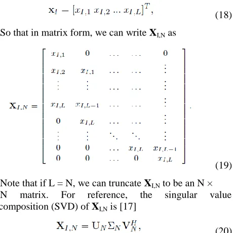
HN [17]. Let xI be a complex, time-varying L × 1 vector,

written as

(18)

So that in matrix form, we can write XI,N as

(19)

Note that if L = N, we can truncate XI,N to be an N ×

N matrix. For reference, the singular value decomposition (SVD) of XI,N is [17]

(20)

Where UN and VN are unitary N × N matrices whose

columns are the eigenvectors of XI,NXHI,N, and ΣN is an

N×N diagonal matrix whose elements are the positive square roots of the eigenvalues of XI,NXHI,N. Here, (·)H

denotes Hermitian (complex conjugate) transpose of the matrix (·).

The Domain Decomposition (DD) of XI,N uses the FrFT

matrix Fa and is defined as [17]

(21)

Where the Λk‟s are matrices whose diagonal elements

contain weighting coefficients similar to the weights ΣN of

Eq. (20).

Fig. 1 shows the WD of the desired signal x(i) and a potential corrupting interferer xI(i).

The optimum FrFT axis tak where the interference can best be filtered out, corresponds to the axis where the projection of the WD of xI(i) is maximum. The WD of a

continuous time signal x(t) can be written as

(22)

Fig. 1. Wigner Distribution of Signal x(i) and Interferer xI(i);

Optimum rotation axis tak

We can now summarize the DD-FrFT algorithm in [15]: It is well-known that the projection of the WD of a signal, specifically the interfering signal xI(t), onto an axis tak gives the energy in the FrFT, |XI,ak(t)|

2

(see e.g. [7] or [8]). Letting αk = akπ/2, this is written as

(23)

So this is the quantity to be maximized. Now, examining Eq. (21), we observe that the amount of energy contained in XI,N in the domain given by ak is given by the coefficient

Λk. Based upon the above, we choose the ak which

maximizes Λk in Eq. (21) and hence the energy of the

interferer. We then rotate to this domain to best filter the interferer out. Thus, the problem is to determine the maximum Λk in Eq. (21). The solution is a maximization

problem, written as [15]

(24)

So that the value of ak which produces the largest Λk is

International Journal of Emerging Technology and Advanced Engineering

Website: www.ijetae.com (ISSN 2250-2459, ISO 9001:2008 Certified Journal, Volume 6, Issue 10, October 2016)

49

V. WIGNER DISTRIBUTION METHOD

The WD technique presented in [16] estimates the optimum value of „a‟ without using the received signal y(i), because this signal contains the SOI and interference together, without needing a large number of samples N, and without matrix inversions [16]. Referring back to Fig. 1, note that we can choose the FrFT rotational axis as that for which the desired signal and interference do not overlap, or in the practical case, overlap as little as possible. To avoid computing the WD of the SOI and interferer (i.e. SOI turned off) separately, which is difficult in practice, this method recognizes that we can more easily compute the WD along each axis ta by computing the energy of the

FrFT along that axis [16]. Hence, this algorithm computes the energy of the FrFT of both the SOI and interference, computes their product, sums the values over the new time-frequency axis ta defined by the rotational parameter „a‟,

and selects as the optimum „a‟ the value for which the result is minimum. The algorithm is summarized as follows [16]: For 0 < a < 2, compute

(25)

(26)

and

(27)

Choose the value of „a‟ for which ℜXXI(a) in Eq. (27) is minimum. Recall that Fa was defined in Eq. (4). Again, note that the interferer could be replaced with a non-stationary channel, and the algorithm could still be applied. It is also important to mention that computing |XIa(i)|

2 _in

Eq. (26) above requires calculation of the FrFT of the interference. Since the algorithm operates with very few samples, we can compute this in gaps where the SOI is off, e.g. using empty sub-carriers, as in OFDM, etc. [16]. Once we have the best „a‟, we again compute the filter coefficients from Eq. (12), now denoted g0,WD−FrFT and

apply Eq. (8) to obtain the bit estimates.

VI. REDUCED RANK MWFSOLUTION

The full rank MMSE solution in Eq. (12) can be implemented efficiently and with better performance using the correlations subtraction architecture of the multistage Wiener filter (CSAMWF). The MWF was first introduced in [3] − [6] and the efficient CSA implementation of the MWF was first presented in [12].

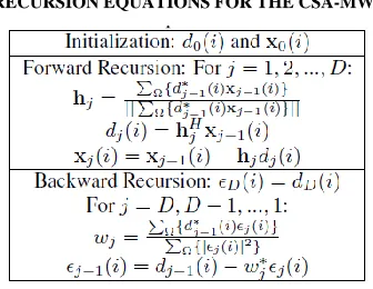
The MWF-FrFT algorithm was introduced in [14]. Referring to [14], we initialize the CSA-MWF with

(28)

and

(29)

Recall that Z(i) was defined in Eq. (16). Using the recursion equations in Table I, the CSA-MWF computes the D scalar weights wj, j = 1, 2,..., D and vectors hj, from

which we form the optimum filter

(30)

Rank reduction is achieved because we set D < N. Again, we search over all „a‟ to find the best one, computing the filter coefficients from Eqs. (28) - (30) and Table I. Hence, this is the only algorithm that applies the MWF filter versus the MMSE filter.

VII. SIMULATIONS

We present simulation examples to compare the performance of the four techniques discussed in this paper: MMSE-FrFT, DD-FrFT, WD-FrFT, and MWF-FrFT, showing the robustness of the latter three methods, with the MWF-FrFT showing the most promise when the Eb/N0 is

very low. After computing the best rotational parameter „a‟ for each algorithm, we compute the filter coefficients using Eq. (12) for the first three algorithms and Eq. (30) for the fourth and then apply them to Eq. (8) to compute the bit estimates. These are compared to the true bit to determine if an error occurs, so we can compute the MSE, given by the cost function in Eq. (10). In the first example we assume the desired BPSK signal is corrupted by a non-stationary chirp interferer signal given in vector form by (see Example 3 in [7])

TABLE I

International Journal of Emerging Technology and Advanced Engineering

Website: www.ijetae.com (ISSN 2250-2459, ISO 9001:2008 Certified Journal, Volume 6, Issue 10, October 2016)

50 (31)

Where fs is an arbitrary sampling rate and we have

dropped the block index i for convenience. We set Eb/N0 =

−5 dB by scaling the amplitude of the AWGN. We vary the CIR, which is the ratio of the desired signal power to the chirp interferer power, from −10 to 10 dB. Here, due to the non-stationarity of the interference, we choose a very small block size for best performance, so we let N1 = 2, SPB = 2,

and therefore N = 4. We let the rank of the MWF-FrFT algorithm be D = 1, since there is only a single desired signal and we have a training sequence. The performance is not very sensitive to rank, so we choose D = 1 for faster computation. Since the sample size (N = 4) is so small, the choice of rank is 1 ≤ D ≤ 4. We search over 0 < a < 2 using a step size of ∆a = 0.01. We run M = 10,000 trials to obtain good statistical averages at each CIR and plot both the best „a‟ and the MSE as a function of CIR in Fig. 2. The subsequent examples use Eb/N0 = 0,5,10, and 15 dB,

respectively, and are shown in Figs. 3 to 6.

From all the figures, we see that all three new algorithms (DD-FrFT, WD-FrFT, and MWF-FrFT) are more robust over a large range of CIR, at low Eb/N0

,

much lower MSE between the signal and its estimate than the conventional MMSE-FrFT algorithm, by up to several orders of magnitude. When Eb/N0 is high, the DD and WD

algorithms are better than the MWF, at low CIR, but the MWF and MMSE perform well too; at high CIR, all four do well. When Eb/N0 is low, however, the MWF is best.

Also, we observe that the best value of „a‟ is different for all four algorithms - it is typically less than 0.05 for the MWF-FrFT, it is about 0.25 for the DD-FrFT and WD-FrFT for this interfering signal, and it varies significantly for MMSE-FrFT (confirming that obtaining a good estimate of the bits is difficult for MMSE-FrFT in the non-stationary environment). Since all four algorithms estimate the best „a‟ using different criteria, differences in the outcome are expected.

Fig. 2. CIR [dB] vs. BER; BPSK SOI + Chirp Interferer; Eb/N0 = −5

dB

VIII. CONCLUSION

In this paper, we study three new algorithms for estimating the optimum rotational parameter „a‟ in the FrFT domain for suppressing interference. The three algorithms are based on domain decomposition of the signal of interest, the relationship of the FrFT to the Wigner Distribution, and the reduced rank MWF. All three greatly outperform conventional MMSE filtering in the FrFT domain and work over a range of CIR and Eb/N0. At low

Eb/N0, MWF is best, but for high Eb/N0 all algorithms

International Journal of Emerging Technology and Advanced Engineering

Website: www.ijetae.com (ISSN 2250-2459, ISO 9001:2008 Certified Journal, Volume 6, Issue 10, October 2016)

51

Fig. 3. CIR [dB] vs. BER; BPSK SOI + Chirp Interferer; Eb/N0 = 0 dB

Fig. 4. CIR [dB] vs. BER; BPSK SOI + Chirp Interferer; Eb/N0 = 5 dB

Fig. 5. CIR [dB] vs. BER; BPSK SOI + Chirp Interferer; Eb/N0 = 10

dB

Fig. 6. CIR [dB] vs. BER; BPSK SOI + Chirp Interferer; Eb/N0 = 15

International Journal of Emerging Technology and Advanced Engineering

Website: www.ijetae.com (ISSN 2250-2459, ISO 9001:2008 Certified Journal, Volume 6, Issue 10, October 2016)

52 REFERENCES

[1] Alieva, T., and Bastiaans, M.J., “Wigner Distribution and Fractional Fourier Transform”, Proc. 6th _{Int. Symposium on Sig. Proc. and its}

Applications, Vol. 1, pp. 168-169, Kuala Lumpur, Malaysia, Aug. 2001.

[2] Candan, C., Kutay, M.A., and Ozaktas, H.M., “The Discrete Fractional Fourier Transform”, IEEE Trans. on Sig. Proc., Vol. 48, pp. 1329-1337, May 2000.

[3] Goldstein, J.S., and Reed, I.S., “Multidimensional Wiener Filtering Using a Nested Chain of Orthogonal Scalar Wiener Filters”, University of Southern California, CSI-96-12-04, Dec. 1996. [4] Goldstein, J.S., and Reed, I.S., “A New Method of Wiener Filtering

and its Application to Interference Mitigation for Communications”, Proceedings of IEEE MILCOM, Vol. 3, pp. 1087-1091, Monterey, CA, Nov. 1997.

[5] Goldstein, J.S., Reed, I.S., and Scharf, L.L, “A New Method of Wiener Filtering”, Proc. 1st AFOSR/DSTO Workshop on Defense Applications of Sig. Proc., Victor Harbor, Australia, Jun. 1997. [6] Goldstein, J.S., Optimal Reduced Rank Statistical Signal Processing,

Detection, and Estimation Theory, Ph.D. Thesis, Dept. of Elec. Eng., Univ. Southern California, Los Angeles, CA, Dec. 1997.

[7] Kutay, M.A., Ozaktas, H.M., Arikan, O., and Onural, L., “Optimal Filtering in Fractional Fourier Domains”, IEEE Trans. on Sig. Proc., Vol. 45, No. 5, May 1997.

[8] Kutay, M.A., Ozaktas, H.M., Onural, L., and Arikan, O. “Optimal Filtering in Fractional Fourier Domains”, Proc. IEEE Int. Conf. on Acoustics, Speech, and Signal Proc. (ICASSP), Vol. 2, pp. 937-940, 1995.

[9] Lin, Q., Yanhong,Z., Ran, T., and Yue, W., “AdaptiveFiltering in Fractional Fourier Domain”, Int. Symposium on Microwave, Antenna, Propagation, and EMC Technologies for Wireless Comm. Proc., pp. 1033-1036, 2005.

[10] Ozaktas, H.M., Zalevsky, Z., and Kutay, M.A., “The Fractional Fourier Transform with Applications in Optics and Signal Processing”, John Wiley and Sons: West Sussex, England, 2001. [11] Reed, I.S., Mallett, J.D., and Brennan, L.E., “Rapid Convergence

Rate in Adaptive Arrays”, IEEE Transactions on Aerospace and Electronic Systems, Vol. 10, pgs. 853-863, Nov. 1974.

[12] Ricks, D.C., and Goldstein, J.S., “Efficient Architectures for Implementing Adaptive Algorithms”, Proc. of the 2000 Antenna Applications Symposium, pgs. 29-41, Allerton Park, Monticello, Illinois, Sep. 20-22, 2000.

[13] Subramaniam, S., Ling, B.W., and Georgakis, A., “Filtering in Rotated Time-Frequency Domains with Unknown Noise Statistics”, IEEE Trans. on Sig. Proc., Vol. 60, No. 1, Jan. 2012.

[14] Sud, S., “Performance of Adaptive Filtering Techniques Using the Fractional Fourier Transform for Non-Stationary Interference and Noise Suppression”, Int. J. of Enhanced Research in Sci., Tech., & Eng. (IJERSTE), Vol. 4, No. 10, pp. 116-122, Oct. 2015.

[15] Sud, S., “Estimation of the Optimum Rotational Parameter for the Fractional Fourier Transform Using Domain Decomposition”, Int. J. of Recent Dev. in Eng. and Tech. (IJRDET), Vol. 4, No. 9, pp. 6-11, Sep. 2015.

[16] Sud, S., “Estimation of the Optimum Rotational Parameter of the Fractional Fourier Transform Using its Relation to the Wigner Distribution”, Int. J. of Emerging Tech. and Adv. Eng. (IJETAE), Vol. 5, No. 9, pp. 77-85, Sep. 2015.