Forecast of fund volatility using least squares wavelet support vector regression machines

Journal of Chemical and Pharmaceutical Research, 2014, 6(6):190-195

Research Article

ISSN : 0975-7384

CODEN(USA) : JCPRC5

Forecast of fund volatility using least squares wavelet support vector

regression machines

Li-Yan Geng* and Yi-Gang Liang

School of Economics and Management, Shijiazhuang Tiedao University, Shijiazhuang, China

_____________________________________________________________________________________________

ABSTRACT

The forecasting of financial volatility is important for asset management and portfolio selection. It is difficult to forecast financial volatility accurately due to the high nonlinearity and clustering in financial volatility sequences. To improve the forecasting accuracy for financial volatility, Least squares wavelet support vector regression machines (LS-WSVR) is applied to forecasting financial volatility. Using daily SZSE fund index data from China stock markets and selecting three different kinds of wavelet kernel functions, the paper demonstrates the validity of LS-WSVR for fund volatility forecasting. Four statistical indices, RMSE, MAE, LL, and LINEX, are adopted to test the forecasting performance of LS-WSVR. Experimental results show that on the whole LS-WSVR with three different wavelet kernel functions outperforms the LS-SVR with Gaussian kernel function for in-sample and out-of-sample fund volatility forecasting. Moreover, the forecasting performance of LS-WSVR with Morlet kernel function is better than those of LS-WSVR with Mexican hat wavelet kernel function and DOG wavelet kernel function.

Keywords: Fund volatility; Forecasting; Least squares wavelet support vector regression machines

_____________________________________________________________________________________________

INTRODUCTION

The difficulty of financial volatility forecasting is well known since financial volatility is characterized by the high nonlinearity, clustering, and fat tail. In the last few years, researchers have continued to construct different models to forecast financial volatility. The traditional econometric models, such as regression model and autoregressive model, have difficulty to model these characteristics of volatility. ARCH model suggested by Engle can model the characteristics of volatility well [1]. As the generalized form of ARCH model, GARCH model and has been widely recognized and been proven to be effective for volatility forecasting [2-3].

Recent years, artificial intelligence approach was introduced into the volatility forecasting area to further improve the forecasting performance of the traditional volatility forecasting model, in which neural network (NN) is a typical representative. Typically, NN was combined with GARCH model to forecast volatility [4-5]. The results show that NNs improve the volatility forecasting accuracy of GARCH model due to their data-driven nonparametric and nonlinear properties. However, NN is not perfect and the application of NN often suffers from problems, such as local minima, the dimension curse and over-learning, which has limited the popularization and application of NN.

Least squares support vector machines (LS-SVM), developed by Suykens and Vandevalle, is an improved type of SVM [12]. By substituting equality constraints for the original quadratic programming, LS-SVM reduces the complexity of computation. Usually, LS-SVM is used for classification and recognition. Another form of LS-SVM, Least squares support vector regression machines (LS-SVR), is used for regression analysis and forecasting. Until now, some researchers have adopted LS-SVR to forecast volatility under the GARCH-type and CARRX framework and their research results have shown good forecasting performance [13-15].

The generalization performance of LS-SVR is mainly depends on the selection of an appropriate kernel function.

Gaussian kernel has been generally used in LS-SVR because of its good generalization ability. However, Gaussian

kernel can’t make LS-SVR approach any curve in L2(Rn) space, which lead LS-SVR can’t approximate arbitrary

objective function. Least squares wavelet support vector regression machines (LS-WSVR) is a type of LS-SVR, in which wavelet kernel is used as the kernel function. At the same time, wavelet kernels are also utilized as support vector kernel to improve the generalization performance of LS-SVR[16].

In this paper, LS-WSVR with three different wavelet kernels are applied to forecasting fund volatility, and the in-sample and out-of-sample forecasting performance of these LS-WSVR are compared with those of LS-SVR with

Gaussian kernel functions according to evaluation indices. The remaining of this paper is organized as follows.

Section 2 presents the theory of LS-WSVR algorithm. Empirical results on SZSE fund index illustrating the effectiveness of the LS-WSVR are provided in Section 3. Conclusions are given in the final section.

EXPERIMENTAL SECTION

Least squares wavelet support vector regression machines

LS-SVR applies a squared loss function to replace to a QP problem and obtains solutions by solving linear equations. In this paper, a one-step-ahead forecasting model of LS-SVR is established to avoiding the cumulative errors from the previous step.

Support one time series

1 2

{ , ,..., }l

D= x x x with l training samples, based on a nonlinear mapping function j ,

t

x Î Ris mapped into a high-dimensional feature space in which the one-step-ahead forecasting model is defined as:

1 ( ) T

t t

x₊ =w j x +b, t=1, 2,...,l-1. (1) where ω is weight vector and b is bias term. Then, we obtain the optimization problem of LS-SVR as:

1

2 2

, , ₁

1

1 min ( , , )

2 2

s.t. ( ) 1, 2, , 1

l

t

b _t

T

t t t

J b

x x b t l

w x

g

w x w x

w j x

-= + = + = + + =

-å

L

|| || ₍₂₎

with

t R

x Î is error vector and γ is a positive constant named regularization parameter. In order to solve the above optimization problem, Lagrange multipliers

t R

a Î (t=1, 2, …, l-1) are introduced and the lagrangian function is defined as: 1 1 1 ( , , , ) ( , , ) ( ( ) ) l T

t t t t

t

Lwbx a J wbx a w j x b x x

-+ =

= -

_å

+ + - (3)

On the basis of Karush-Kuhn-Tucker (KKT) condition, the conditions for optimality are given by:

1 1 1 1 1

( ) 0

0

0, 1,2,..., 1

( ) 0 1, 2,..., 1

l t t t l t t t t t T

t t t

t L x L b L

e t l

e

L

x b e x t l

w a j

w a a g w j a -= -= + ì ¶ = - = ï ï ¶ ï ¶

ï _{= =}

ï_¶ ï í_¶

ï _{= - = =}

-ï ¶ ï ï ¶

ï _{= + + - = =}

-ï ¶ î

å

å

(4)

After eliminating ζ and ω, it can be obtained a set of linear equations:

0

T

0

l l

b

E

E

g

_´

é

ù é ù é ù

ê

ú ê ú ê ú

=

ê

ú ê ú ê ú

ë

Ω

+ I /

û ë û ë û

α

1

(5)

______________________________________________________________________________

kernel function. Then, the one-step-ahead forecasting model of LS-SVR is given by

1 1 , 1 ( ) l

t j t j

t j

x a x ,x b

-+ =

=

_å

K + (6) For LS-SVR, the kernel functions, which satisfy Mercer’s theorem, are admissive support vector kernel functions. There are two kinds of kernels that can be used as the kernel function of LS-SVR, they are dot product kernels and translation invariant kernels. According to wavelet decomposition and the construction method of kernel function for LS-SVR, the translation invariant kernels that satisfy the translation invariant kernel theorem are as wavelet kernels for LS-SVR: 1 ( , ) ( ) d t j

t j t j

t t

x x x x x x

a j =

æ - ö

ç ÷

= - = _{ç ÷}

è ø

Õ

K K (7)

where φ(x) is called “mother wavelet” and at (at>0) is the scaling parameters of wavelet. Presently, some wavelet

kernels functions have been successfully used in LS-SVR, including Mexican hat wavelet kernel, Morlet wavelet kernel and DOG kernel. Mother wavelet and wavelet kernel function for Mexican hat, Morlet, and DOG are given in Table 1.

Table 1. Mother wavelet and wavelet kernel function

Mother wavelet Wavelet kernel function Mexican hat

(

)

2 2

( ) 1 exp 2

x x x

j = - æç_ç- ö÷_÷ è ø

2 2

2 2

1

|| || || ||

( , ) 1 exp

2

d

t j t j

t j

t t t

x x x x

x x

a a

=

æ _- ö æ _- ö

ç ÷ ç ÷

= -

-ç ÷ ç ÷

è ø è ø

Õ

K

Morlet 2

( ) cos(1.75 ) exp 2

x

x x

j = æç_ç- ö÷_÷

è ø

2

2 1

1.75 || || || || ( , ) cos( ) exp

2 d

t j t j

t j

t t t

x x x x

x x

a a

=

æ ö

æ - ö _ç - _÷

ç ÷

= _{ç ÷}

-ç ÷

è ø è ø

Õ

K

DOG 2 2

1 ( ) exp exp

2 2 8

x x

x

j = çæ_ç- _÷ö÷- æ_çç- ÷ö_÷

è ø è ø

2 2

2 2

1

|| || 1 || ||

( , ) exp exp

2 2 8

d

t j t j

t j

t t t

x x x x

x x

a a

=

ì æ _- ö æ _- öü

ï _{ç ÷ ç ÷}ï

= í _ç- _÷- _ç- _÷ý

ï _{è ø è ø}ï

î þ

Õ

K

RESULTS AND DISCUSSION

Data description

The used data is daily closing prices for SZSE fund index of China stock market from January 4, 2011 through December 13, 2012. According to a traditional approach, the continuously compounded daily returns are obtained by the logarithmic difference of daily closing prices multiplied by 100. That is,

y_t =100´

₍

logp_t-logp_t-1

₎

(8)

where yt is the continuously compounded daily returns, pt is the daily closing price at time t. The data set is divided

into two subsets: the first subset of the data (from January 4, 2011 through March 29, 2012) is the forecasted in-sample period, and the second subset of the data (from March 30, 2012 through December 13, 2012) is the forecasted out-of-sample period.

The true underlying volatility process ht2 is an unobservable stochastic quantity. The most common method for

measuring a volatility is to square the observed returns. In this paper, the squared return yt

2

is employed as a measurement for the unobservable volatility process. Replacing xt in (6) as yt2, the LS-WSVR for forecasting

volatility will be constructed.

Empirical process

To validate the volatility forecasting performance of LS-WSVR, three kernel functions: Mexican hat wavelet kernel,

Morlet wavelet kernel and DOG wavelet kernel are selected as the kernel function in LS-WSVR respectively and the

three LS-WSVR models are used to forecast fund volatility. For simplicity, we suppose at =a, such that the number

of parameters needed in LS-WSVR becomes only two: the regularization parameter γ and the scaling parameter a. In

order to avoiding the cumulative errors from the previous step, the models established based on the optimal parameters is used to obtain one-step-ahead volatility forecasts of SZSE fund returns.

For comparison, one-step-ahead in-sample and out-of-sample forecasting results from LS-WSVR based three wavelet kernel functions are compared with LS-SVR based Gaussian kernel function, respectively. And Gaussian kernel function is defined as:

2

2

|| ||

( , ) exp

2 t j t j x x x x s

æ _- ö

ç ÷

= _ç- _÷

è ø

where σ2 is the kernel parameter. Consequently, there are only two parameters: the regularization parameter γ and σ2 needed in LS-SVR with Gaussian kernel function.

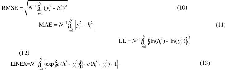
Four statistical metrics are used to compare forecasting performance of different models, including root mean squared error (RMSE), mean absolute error (MAE), logarithmic error statistic (LL), and linear-exponential (LINEX). These statistics are defined as follows:

1 2 2 2 1

RMSE ( )

N

t t

t

N- y h

=

=

_å

- (10)

1 2 2

1

MAE

N

t t

t

N- y h =

=

_å

- (11)

2

1 2 2

1

LL ln( ) ln( )

N

t t

t

N- h y

=

é ù

=

_å

_ë - _û

(12)

{

}

1 2 2 2 2

1

LINEX= exp ( ) ( ) 1

N

t t t t

t

N- c h y c h y

=

é _- ù_{- -}

-ë û

å

(13)

where 2

t

h is the forecasted volatility and 2 t

y is the realized volatility measured through the squared returns in the period of t. N is the number of the observations. RMSE, MSE are symmetric loss functions and LL and LINEX are asymmetric loss functions. The smaller loss function implies the better forecasting performance.

RESULTS AND DISCUSSION

The results on in-sample forecasting results for SZSE fund volatility are listed in Table 2, where LS-WSVR1, LS-WSVR2, and LS-WSVR3 stands for LS-WSVR with Mexican hat kernel function, Morlet kernel function, and

[image:4.595.171.536.154.268.2]

DOG kernel function, respectively. LS-SVR stands for LS-SVR with Gaussian kernel function.

Table 2. RMSE, MAE, LL, LINEX of in-sample volatility forecasts by four models

Loss functions LS-WSVR1 LS-WSVR2 LS-WSVR3 LS-SVR RMSE 1.1639 1.1636 1.1646 1.1658

MAE 0.9318 0.931 0.9332 0.9376 LL 8.9089 8.9084 8.9208 8.9386 LINEX 1.1281 1.088 1.181 1.1676

As is shown in Table 2, LS-WSVR1 and LS-WSVR2 provide the smaller statistics RMSE, MAE, LL and LINEX than LS-WSVR3 and LS-SVR. As for LS-WSVR3 and LS-SVR, apart from LINEX index, LS-WSVR3 has smaller RMSE, MAE and LL than LS-SVR. That is to say, LS-WSVR on the whole produces superior in-sample volatility forecasting results relative to LS-SVR. We can also see from the results of Table 2 that LS-WSVR2 has better in-sample volatility forecasting results than LS-WSVR1 and LS-WSVR3.

The results on out-of-sample forecasting for SZSE fund volatility from the four models are given in Table 3. It shows that the four statistical metrics RMSE, MAE, LL, and LINEX of LS-WSVR1, LS-WSVR2, and LS-WSVR3 are all smaller than ones of LS-SVR, indicating that LS-WSVR are superior to LS-SVR on out-of-sample volatility forecasting ability. The main reason for the outperformance of LS-WSVR to LS-SVR is that wavelet kernel functions can approximate arbitrary objective function well due to their multi-resolution property.

Table 3. RMSE, MAE, LL, LINEX of out-of-sample volatility forecasts by four models

Loss functions LS-WSVR1 LS-WSVR2 LS-WSVR3 LS-SVR

RMSE 1.0093 1.0092 1.0114 1.0128 MAE 0.733 0.7318 0.7355 0.7375 LL 9.907 9.9001 9.9251 9.9386 LINEX 1.4469 1.4731 1.5309 1.571

As for three LS-WSVR models, with the exclusion of LINEX index, LS-WSVR2 performs better than LS-WSVR1 and LS-WSVR3 on out-of-sample volatility forecasting. And for LINEX index, LS-WSVR1 seems to have superior volatility forecasts relative to LS-WSVR2 and LS-WSVR3.

______________________________________________________________________________

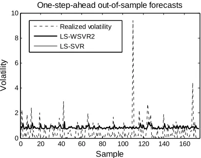
[image:5.595.186.393.94.260.2]

Morlet wavelet kernel function performs the best among the three LS-WSVR models.

Figure 1. Comparison of in-sample volatility forecasts of SZSE fund index for two models

One-step-ahead in-sample and out-of-sample volatility forecasts from LS-WSVR based Morlet wavelet kernel (LS-WSVR2) and LS-SVR based Gaussian kernel (LS-SVR) are shown in Figure 1 and Figure 2, respectively.

Figure 2. Comparison of out-of-sample volatility forecasts of SZSE fund index for two models

According to the figures, volatility forecasts provided by both models are all close to the mean of the realized volatility. Compared with LS-SVR, LS-WSVR2 captures some up and down peaks in the realized volatility series well. Therefore, it is concluded that LS-WSVR2 is an effective method for volatility forecasting.

CONCLUSION

This paper applies LS-WSVR based three different kernel functions to forecasting fund volatility. In-sample and out-of-sample forecasting results of the three models are compared with those of LS-SVR based Gaussian kernel function. Empirical evidence on SZSE fund index from China stock market indicates that LS-WSVR based three wavelet kernels functions are all superior to the Gaussian-kernel LS-SVR in term of volatility forecasting accuracy. And LS-WSVR based Morlet kernel function offers better volatility forecasting performance than LS-WSVR based

Mexican hat kernel function and DOG kernel function, respectively.

Acknowledgements

This work was supported by the Scientific Research Foundation of the Ministry of Education of China for Young Scholars “Intelligent Forecasting Methods for Financial Volatility and Its Empirical Research” (No. 11YJC790048).

REFERENCES

[1]RF Engle. Econometrica, 1982, 50(4): 987-1008.

[2]T Bollerslev. Journal of Econometrics, 1986, 31(3): 307-327.

[3]JP Morgan; Reuter. RiskMetrics-Technical Document, 4th Edition, Morgan Guaranty Trust Company, New York,

1996; 63-70.

0 50 100 150 200 250 300

0 2 4 6 8 10

Sample

V

o

la

ti

li

ty

One-step-ahead in-sample forecasts

Realized volatility LS-WSVR2 LS-SVR

0 20 40 60 80 100 120 140 160

0 2 4 6 8 10

Sample

V

o

la

ti

li

ty

One-step-ahead out-of-sample forecasts

[image:5.595.187.393.318.480.2]

[4]RG Donaldson; M Kamstra. Journal of Empirical Finance, 1997, 4(1): 17-46. [5]B Melike; OE Ozgür. Expert Systems with Applications, 2009, 36(4): 7355-7362. [6]VN Vapnik. IEEE Transactions on Neural Networks, 1999, l0(5): 988-999. [7]SY Chen; WK Härdle; K Jeong. Journal of Forecasting, 2010, 29(4):406-433.

[8]BH Wang; HJ Huang; XL Wang. Neural Computing and Applications, 2013, 22: 21-28. [9]VV Gavrishchaka; B Supriya. Computational Management Science, 2006, 3(2):147-160. [10]PC Fernando; AAR Julio; G Javier. Quantitative Finance, 2003, 3(3): 167-172. [11]LB Tang; HY Sheng; LX Tang. Systems Engineering, 2009, 27(1): 87-91. [12]JAK Suykens; J Vandevalle. Neural Processing Letters, 1999, 9(3): 293-300. [13]PH Ou. International Journal of Economics and Finance, 2010, 2(1): 51-64. [14]LY Geng; F Yu. Journal of Applied Sciences, 2013, 13(22): 5132-5137