State Feedback Control Based Networked Control System
Design with Differential Evolution Algorithm
Ti-Hung Chen
1,*, Ming-Feng Yeh
21Department of Computer Information and Network Engineering, Lunghwa University of Science and Technology, Taiwan 2Department of Electrical Engineering, Lunghwa University of Science and Technology, Taiwan
Copyright©2017 by authors, all rights reserved. Authors agree that this article remains permanently open access under the terms of the Creative Commons Attribution License 4.0 International License
Abstract
This paper will propose the state feedbackcontrol based networked control system (NCS) design with the differential evolution algorithm. For designing a networked control system, one has to overcome the problems about the random latency and the data packet dropouts. Here, we will apply the state feedback control theory to design a controller to overcome the random latency and the data packet dropouts of NCS and guarantee the stability of the overall system. To improve the control performance, the differential evolution algorithm (DE) is applied to search the optimal control parameters. In this way, one can design NCS more effectively and without need to solve a complex Lyapunov-Krasovskii stability criterion. Finally, computer simulations are given to demonstrate the proposed control strategy and to illustrate its effectiveness.
Keywords
Networked Control System, DifferentialEvolution Algorithm, Packet Dropouts, Time Delay, State Feedback Control
1. Introduction
The Internet of Things (IoT), the important technology of industry 4.0 [1-3], is emerging as the next technology mega-trend. Lots of researchers and research organization make studies about IoT [4-7]. An important issue of IoT is the networked control systems (NCSs) design [8-15], which is a spatially distributed system for which the connection between sensors, actuators, and controllers is supported by share communication networks. In NCS, data are transmitted in an atomic unit called data packets. It means that the system states and the output signals are sampled by the sensors and transmitted to the controllers by the data packets, and the controller signals are transmitted to the actuators by the data packets, and the actuators would control the controlled plants according to the receiving data packets.
Due to the introduction of the share communication network, two major challenges in NCSs still to be fully addressed are the effects of both “latency (caused by
propagation, transmission, router, processing, computer … etc.)” and “packet dropout (caused by network congestion, multi-path fading, faulty network drivers… etc.)” on the system performance [14]. To treat the mentioned effects, several methods have been proposed. Seiler et al. adopted the H∞control theory to stabilize NCS and analyzed the system robustness [9, 13]. Huang and Nguang applied the state feedback controller to treat the control problem of NCS [10]. Peng et al. applied T-S fuzzy control technique to guarantee the stability of NCS [11, 13]. Sahoo and Jagannathan applied stochastic control theory and event- driven technique to optimize the NCS design [15].
From the above-mentioned method, we can find out that designing NCS, one usually analyzes the stability of NCS based on Lyapunov stability theorem and solve the Lyapunov-Krasovskii stability criterion to obtain the control gain matrix [9-11, 14]. But, generally, the Lyapunov- Krasovskii stability criterion is difficultly calculated. So that, this paper adopted the differential evolution (DE [16-18]) is applied to search the optimal control gain matrix effectively.
Since in 1995 Storn and Price proposed the differential evolution (DE, [16]), which has attracted a lot of research interests. The advantage of DE is that their convergence rate is faster than many other acclaimed global optimization methods. Otherwise, it requires few control variables, is robust, easy to use, and lends itself very well to parallel computation. Hence it is very promising to solve lots of engineering optimization problems. Guney and Basbug adopted DE into antenna design [19]. Zheng et al. applied DE to estimate the state of hybrid power system [20]. Applied DE to microwave circuit designs [21].
In this paper, we adopt DE into NCSs design. First, we design the state feedback controller to overcome the latency and the packet dropout of NCS. Then, to optimize the control performance, DE is applied to search the optimal parameters of the controller and to guarantee the stability of the overall system. Finally, the computer simulations are given to demonstrate the effectiveness of the proposed results.
follows: First, the controller design for NCS with transmission delay and data packet dropout is obtained and the stability of the overall system can be guaranteed. Also, by using DE, without solving the difficult Lyapunov- Krasovskii stability criterion, the optimal control parameters are searched to improve the control performance.
This paper is organized as follows: In section 2, we will describe the system description of NCS. Section 3 will present the design of differential evolution based networked control system. In section 4, computer simulation will be given to illustrate the control performance of the proposed control strategy. Section 5 will conclude this paper.
2. The System Description of NCS
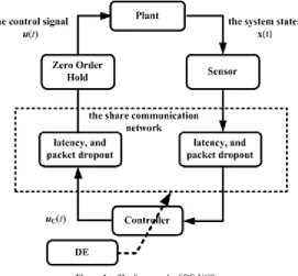
This paper considers a class of the networked control system, where the framework shown in Figure 1 [9]. This system is composed of the following five parts: a sensor, a controller, a zero-order-holder (ZOH), applied as an actuator, a controller, a communication network channel, and a controlled plant.
Consider the controlled plant as following [14]: ) ( ) ( ) ( ) ( )
(t Ax t Axt But ωt
[image:2.595.171.443.233.484.2]x = +∆ + + (1)
Figure 1. The framework of DE-NCS.
where x(t)=[x(t),x(t),...,x(n)(t)]∈ℜn is the state vector, u(t)∈ℜm is the control signal, ω(t)∈ℜn is the unknown external disturbance, A∈ℜn×n and B∈ℜn×m are known constant matrices, and ∆A∈ℜn×n is unknown uncertainty matrix. The initial condition of controlled plant is given as x(t0)=x0. Without loss of generality, we make the following assumption [9]:
Assumption 1: (A,B) is controllable pair.
Assumption 2: The external disturbance ω(t) is bounded. That is, ω(t)∈L2[0,tf], ∀tf ∈[0,∞).
Assumption 3: There exists bounding matrix ElA such that ∆AT∆A≤ETlAElA.
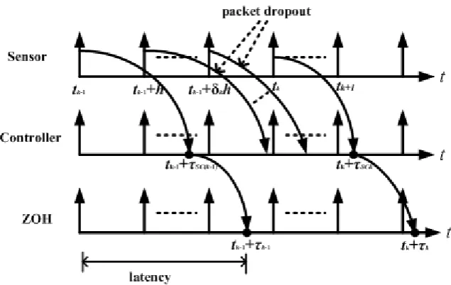
For NCS, since the controller is connected with the sensor or ZOH via a share communication network channel, propagation, transmission, router, processing, computer, storage delays … etc. would cause latency. Also, network congestion, multi-path fading, faulty network drivers would cause packet dropout. Figure 2 show latency and packet dropout of NCS. Because of latency and packet dropout, packets are transmitted from the sensor to the controller spend
sck
τ , and from the controller to the actuator spend τczk. Define the total latency as τk =τsck +τczk at every sampling instant tk and make the following assumptions:
Assumption 4 [14]: The total latency τk is bounded.
Also, for the packet dropout, we make the following assumption:
Assumption 5 [14]: The packet dropout number ηk is bounded as 0≤ηk≤ηmax where ηmax is upper bound of ηk.
Figure 2. Latency and packet dropout of NCS.
To treat the objective, we adopt state feedback control and design the control law as follows:
) ( ) (t Kx t
u = (2) where K is the control gain matrix. Usually, the control gain matrix K is obtained by solving the Lyapunov- Krasovskii stability criterion. But, solving the stability criterion usually has to calculate the difficult LMI problem or an eigenvalue problem. In order to obtain the control gain matrix K more efficiently, this paper applied the differential evolution. The detail algorithm will be provided in Section 3.
3. The Design of Differential Evolution
Based Networked Control System
In this section, we will propose the design of differential evolution based networked control system. Based on the above-mentioned discussion, we will apply DE to search the optimal control gain matrix for NCS. The detail algorithm can be described as follows:Initiation: At first, let the mutation scale factor as F, the crossover rate as Cr, the population size as Np, and the maximum generation number as Gmax . Since
n m× ℜ ∈
K , we randomly generate n m i,1∈ℜ ×
K for i= ,12,..,Np (3) as a population for the 1st generation. Define the fitness function as
∑
+ =
x K
1 1 )
( i,G
f , (4)
and calculate the fitness value for all Ki,G (i= ,12,..,Np). Mutation: Then, randomly select Kr1,G, Kr2,G, and
, , 3G r
K from {K1,G,K2,G,...,KNp,G} and get the mutant vector by the following equation:
) ( 2, 3, ,
1 , 1
,G V r G r G r G
i K F K K
K + = + ⋅ − (5)
Crossover: After that, to increase the diversity of the perturbed parameter vectors, crossover is introduced. Each element of the trial vector, Ki,G+1,U can be get by
otherwise
rand(0,1) if
, ,
, 1 , , 1
, r
U G ji
U G ji U G
ji k C
k
k ≤
= +
+ (6)
Selection: To decide whether or not it should become a member of generation G+1, the trial vector Ki,G+1,U is compared to the target vector Ki,G using the greedy criterion. If vector Ki,G+1,U yields a smaller cost function value than Ki,G, then Ki,G+1 is set to Ki,G+1,U; otherwise, the old value Ki,Gis retained.
In summary, the proposed control strategy can be expressed as the following procedures:
Design Procedures:
Generate Np individuals of the initial population randomly.
for G=1:Gmax do
for i=1:Npdo
calculate the fitness value f(Ki,G)
end for for i=1:Npdo
//Mutation
randomly select Kr1,G,Kr2,G,and Kr3,G, compute Ki,G,V =Kr1,G +F⋅(Kr2,G −Kr3,G) //Crossover
for j=1:(m×nL)do
if rand(0,1)≤Cr, V G ji U G ji k
k , , = , ,
else G ji U G ji k
k , , = ,
end if end for
//selection
if f(Ki,G,U)≥ f(Ki,G)
U G i G
i, 1 K, ,
K + =
else
G i G i, 1 K,
K + =
end for end for
4. Simulation
In this section, an inverted pendulum system simulated as the controlled plant to demonstrate the performance of the proposed control strategy. Let x1(t)be the angular of the pendulum with respect to the vertical line and u(t) be the applied the control signal. Define (t) [x (t),x (t)]T
1 1 = x , )] ( ), (
[x1 t x2 t T
= x(t) = [x1(t), ẋ1(t)]T=
[x1(t), x2(t)]T the dynamic equations of the inverted
pendulum system can be described as follows:
) ( ) ( cos ) 3 / 4 ( ) cos( ) ( cos ) 3 / 4 ( ) cos( ) sin( ) sin( ) ( ) ( ) ( 1 2 1 1 2 1 1 2 2 1 2 2 1 t x l am l u x a x l am l x x lx am x g t x t x t x p p p ω + − + − − = = (7)
where a m m ,g 9.8m/s2
p
c+ =
= is the acceleration due to
gravity, mc is the mass of the cart, mp is the mass of the pole and l is the half length of the pole. In this simulation, we set mc =1kg., mp =0.1kg., l=0.5m. and the sampling period as 0.001sec.
The Jacobian linearized model around the equilibrium T ] 0 , 0 [ ) 0 ( =
x can be obtained directly from x(t) = [x1(t), ẋ1(t)]T= [x1(t), x2(t)]Tthe dynamic equations (Eq.
8), which yields
+ − + ∆ + − = ) ( 0 ) 3 / 4 ( 0 ) ( ) ( ) ( ) ( 0 ) 3 / 4 ( 1 0 ) ( ) ( 2 1 2 1 2 1 t u l am l a t x t x t x t x l am l g t x t x p p ω A (8)
where
∆
A
is be regarded as the uncertainty terms due to latency, packet dropout and linearization error.To demonstrate the proposed method, we simulation the following cases:
Case 1: This case is the ideal condition. It means the
0
A=
∆ , the total latency τk =0, and the packet dropout number
η
k =0. Set the initial condition is as x(0)=[0.2,0]T.Case 2: The total latency is set as the random number generated from a Gaussian distribution with zero mean and the standard deviation as 0.06 sec. The upper bound of total latency τk is set as 0.1. The packet dropout number is set as the random number generated from uniform Gaussian distribution with zero mean and the standard deviation as 1. The bound of
η
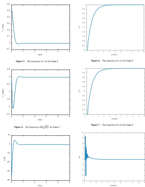
k is set as 15. The initial condition is set as x(0)=[−0.2,0]T. Here we set the mutation scale factor F=0.9 , the crossover rate Cr =0.3, the population size Np=50, and the maximum generation number Gmax =100 for all cases. Besides, in the simulations, all the programs coded by Matlab version R2015a were executed by a personal computer with Intel(R) Core(TM) i7-4600U CPU @ 1.6 GHz processor, 16GB RAM and 64bit-Windows 7 operating system with service pack 1.By the proposed method, we obtain the optima control gain matrix for Case 1 as K=[ -78.2449, -67.9172]. The trajectory of x1(t) and x2(t) are shown in Figure 3 and
Figure 4, respectively, and the control signal u(t) is Figure 5. For Case 2, we get the optima control gain matrix as
26.0754] 43.6987, [ =
K . Figure 6-8 shown the
trajectory of x1(t), the trajectory of x2(t) and the control
Figure 3. The trajectory of x1(t) for Case 1
Figure 4. The trajectory of
x
2(t)
for Case 1 [image:5.595.53.543.77.708.2]Figure 5. The control signal u(t) for Case 1
u(t)
Figure 6. The trajectory of x1(t) for Case 2
Figure 7. The trajectory of x2(t) for Case 2
Figure 8. The control signal u(t) for Case 2
time
0 1 2 3 4 5
x (rad)1
-0.1 0 0.1 0.2 0.3 0.4 0.5 0.6
time
0 1 2 3 4 5
x (rad/s)2
-2.5 -2 -1.5 -1 -0.5 0 0.5
time
0 1 2 3 4 5
u (N)
-40 -30 -20 -10 0 10
time(sec)
0 1 2 3 4 5 6 7 8 9 10
x(t)1
-0.2 -0.18 -0.16 -0.14 -0.12 -0.1 -0.08 -0.06 -0.04 -0.02 0
time(sec)
0 1 2 3 4 5 6 7 8 9 10
x(t)2
-0.2 -0.18 -0.16 -0.14 -0.12 -0.1 -0.08 -0.06 -0.04 -0.02 0
time(sec)
0 1 2 3 4 5 6 7 8 9 10
u(t)
5. Conclusions
This paper has presented the state feedback control based networked control system design with DE algorithm. The state feedback controller is designed to compensate the latency, and packet dropout and to guarantee the stability of the overall system. Applying DE, the optimal control parameters are searched to improve the control performance.
The main contributions of this paper are briefed as follows: First, the controller design for NCS with transmission delay and data packet dropout is obtained and the stability of the overall system can be guaranteed. Also, by using DE, the optimal control parameters are obtained without solving the difficult Lyapunov-Krasovskii stability criterion, one can obtain the optimal control parameters. The simulation results show that the proposed control strategy can successfully stability the NCS and has good performance. Currently, the proposed control strategy is being studied for the practice systems, although still exist various challenging issues.
Acknowledgements
This work was supported in part by Ministry of Science and Technology, Taiwan, R.O.C. under Grant MOST 105-2221-E-262-016 –
REFERENCES
[1] H. Kagermann, W. Wahlster, J. Helbig, Recommendations for implementing the strategic initiative Industrie 4.0: Final report of the Industrie 4.0 Working Group, 2013.
[2] S. Wang, J. Wan, D. Li, C. Zhang, Implementing smart factory of industrie 4.0: an outlook, International Journal of Distributed Sensor Networks. Vol. 12, No. 1, 1-10, 2016. [3] M. Hermann, T. Pentek, B. Otto, Design Principles for
Industrie 4.0 Scenarios, 2016 49th Hawaii International Conference on System Sciences (HICSS), 5-8, 2016.
[4] L. Atzori, A. Iera, G. Morabito. “The internet of things: a survey,” Computer Networks, vol. 54, pp. 2787-2805, 2010. [5] S. Li, L.D. Xu, and X. Wang, “Compressed sensing signal
and data acquisition in wireless sensor networks and internet of things,” IEEE Trans. Ind. Informatics, vol. 9, no. 4, pp. 2177-2186, 2013.
[6] A. Al-Fuqaha, M. Guizani, M. Mohammadi, M. Aledhari, M. Ayyash, Internet of things: a survey on enabling technologies, protocols, and applications, IEEE Communications Surveys & Tutorials, Vol. 17, No. 4, 2347 – 2376, 2015.
[7] X. Larrucea, A. Combelles, J. Favaro, K. Taneja, Software
engineering for the internet of things, IEEE Software, Vol. 34, No. 1, 24-28, 2017.
[8] G.C. Walsh, H. Ye, and L.G. Bushnell, Stability analysis of networked control systems, IEEE Transactions on Control System Technology, Vol. 10, No. 3, 438-446, 2002.
[9] P. Seiler, and R. Sengupta, An H∞ approach to networked
control, IEEE Transactions on Automatic Control, Vol. 50, No 3, 356-364, 2005
[10]D. Huang, and S.K. Nguang, State feedback control of uncertain networked control systems with random time delays, IEEE Transactions on Automatic Control, Vol. 53, No. 3, 829-834, 2008
[11]C. Peng and T.C. Yang, Communication-delay- distribution- dependent networked control for a class of T-S fuzzy systems, IEEE Transactions on Fuzzy System, Vol. 18, No. 2, 326-335, 2010.
[12]H. Wu, L. Lou, C.C. Chen, S. Hirche, and K. Kühnlenz, Cloud-based networked visual servo control. IEEE Transactions on Industrial Electronics, Vol. 60, no. 2, 554-566, 2013.
[13]T.H, Chen. H∞ fuzzy control for a class of networked control
system, Applied Mathematics & Information Sciences, Vol. 9, No. 1L, 133-139, 2015.
[14]J. Qiu, H. Gao, S.X. Ding, Recent advances on
fuzzy-model-based nonlinear networked control systems: a survey, IEEE Transactions on Industrial Electronics, vol. 63, no.2, pp. 1207-1217, 2016.
[15]A. Sahoo, S. Jagannathan, Stochastic optimal regulation of nonlinear networked control systems by using event-driven adaptive dynamic programming, IEEE Transactions on Cybernetics, Vol. 47, No. 2, 425-438, 2017.
[16]R. Storn, and K. Price, Differential evolution - a simple and efficient heuristic for global optimization over continuous spaces, Journal of Global Optimization, Vol. 11, 341–359, 1997.
[17]K. Price, R.M. Storn, J.A. Lampinen, Differential Evolution: A Practical Approach to Global Optimization, Springer, 2005.
[18]S. Das, P.N. Suganthan, Differential evolution: a survey of the state-of-the-art, IEEE Transactions on Evolutionary Computation, Vol. 15, No. 1, 4-31, 2011.
[19]K. Guney, and S. Basbug, Null synthesis of time-modulated circular antenna arrays using an improved differential evolution algorithm, IEEE Antennas and Wireless Propagation Letters, Vol. 12, 817-820, 2013.
[20]V. Basetti and A.K. Chandel. Hybrid power system state estimation using Taguchi differential evolution algorithm. IET Science, Measurement & Technology, Vol. 9, No. 4, 449-466, 2015.