Modeling of heat exchanger by using bio inspired algorithm

Modeling of Heat Exchanger by using Bio-Inspired Algorithm

N. Atiqah Daud

,S. Md Salleh

1

Faculty of Mechanical and Manufacturing Engineering, Universiti Tun Hussein Onn Malaysia 86400, Parit Raja, Batu Pahat, Johor, MALAYSIA

a

[email protected], [email protected] *

Corresponding Author

Keywords: Heat exchanger, Genetic Algorithm, Particle Swarm Optimization, Modelling, Validation test

Abstract: Modelling of heat exchanger helps to define the error that occurs during the operation. Hence by optimizing it using genetic algorithm and particle swarm optimization, the error that occurred could be minimized and compared between both algorithms.The primary objective of this study was to obtain structural model using Autoregressive Moving Average Exogenous (ARMAX) equation. In this study, data from heat exchanger experiment was used to determine the parameter of ARMAX equation. Using genetic algorithm (GA) and particle swarm optimization (PSO), ARMAX parameters are optimized. Hence, the transfer function represents the plant for modelling. Validation test used were autocorrelation and cross-correlation to validate between normalised data input and error. Based on the result obtained, for GA, the input parameters are 0.000214, -0.000728, -0.0020, and -0.000804 while the output parameters are -1.0000, -0.1783, -0.1473 and 0.3248. For PSO, the input parameters are 0.0104, -0.0122, -0.0067 and 0.0118 while the output parameters are -0.4274, -0.1256, -0.1865 and-0.2614. From validation test, GA produced smoother and effective result compared to PSO with less noise exists.

Introduction

Today, the needs for energy and materials savings, as well as economic incentives, have prompted the need to develop more efficient heat exchangers. A preferred approach to the problem of increasing heat exchanger efficiency, while maintaining minimum heat exchanger size and operational cost, is to increase heat exchanger rate. For this project, the real system of heat exchanger that will be used is the shell and tube exchanger type since it offers a great flexibility to meet almost any service requirement.

This study is important to know about the modelling structure of heat exchanger by using ARMAX equation with two different algorithms used to optimize the parameters. From both algorithms, comparison could be made with the least mean squared error produced. The least mean squared error leads the better modelling structure due to the least error could maximize the efficiency of heat exchanger to supply energy.

Heat Exchanger Modelling Structure Operational

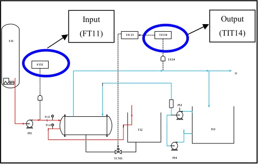
For this study, the experiment is designed to enable good model fit. Since the heat exchanger is closed loop with controller using PID control system, we need to change the closed loop system to open-loop system without the controller. An open-loop control system is controlled directly and only, by an input signal, without the benefit feedback. Figure 1 shows the plant descriptions of heat exchanger.

Figure 1: Plant Descriptions of Heat Exchanger

To start the experiment, Tank 12, Tank 11 and Tank 14 must be filled up with water until the desired level which is at the level of the overflow drain outlet. After that, electric heater at the bottom of the boiler tank, Tank 11 is turned on. The drain valve must be opened so that the water can flow out to the drain. Pump P11, Pump P12 and Pump P14 were discharged. Pump P12 is necessary to pump the water in preheated feedback Tank T12 to Tank T1 After that, the Power Supply (415V/3P) must be switch ON. The TCV11 must be closed. This is to make sure that the shell and tube of the heat exchanger is always filled with medium heating. Then, the Temperature Indicating Controller (TIC11) is set to manual mode while the Level/Flows Indicating Controller is set to automatic mode [6]. After all the above steps are taken, the Recorder LFTR11 is checked to observe the printed data for the input (FT11) and the output (TIT14). When the required number of sampling data is obtained, the output graph is taken for further analysis.

The process of GA consists of selection, crossover and mutation. The rate that used for crossover is 0.67 and mutation rate used in this analysis is 0.001. The mutation rate should be less than 1%. The process will repeatedly continue until a new best generation met. By using PSO, different approach was taken where the position of each agent in PSO is known by position and velocity. At each flight cycle, the objective function is evaluated for each particle, with respect to its current position, and that information is used to measure the quality of the particle and to determine the leader in the subswarms and the entire population [5]. Upper and lower bound were set 0.3 to -0.3 to create the initialize particles positions and velocity randomly. Both position and velocity will be continue updated until its find the best fitness for individual (Pbest) and global fitness (Gbest). The modeling plant of heat exchanger finally obtained in terms of transfer function.

The objectives function of this project is to define the mean squared error (MSE) of the heat exchanger data. The value of mean squared error produced will be differentiating between both algorithms. The least value of MSE produced, the better the modeling of heat exchanger structure. Equation 3 described the mean squared error equation used in this project.

Output

(TIT14) Input

= ∑ − Ŷ

− 2 (3)

Where:

: Normalised output data (woo)

Ŷ : Predicted output (yhat)

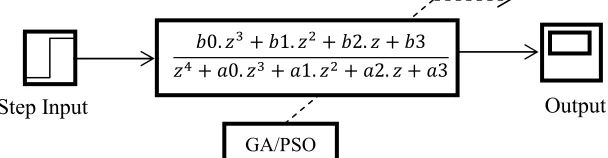
The transfer function obtained will be linked to the plant modelling. To create the plant modelling, standard signal was chose to be the input of model required. The type of standard signal used was step input standard signal. Figure 4 below show the picture of plant modelling for GA and PSO.

Figure 4: Plant modelling for GA and PSO

Results and Discussions

The analysis had been done about 10 times in order to find the best parameters produced. After comparing all the data obtained, the best MSE value for GA found at the fifth analysis. While the best MSE value for PSO found at seventh analysis. Table 1 show the results for parameters obtained from GA and PSO.Table 2 show the transfer function in z-transform obtained from the parameters for both GA and PSO.

Table 1: The results for GA and PSO

No MSE _{a0 a1} a _{a2 a3 b0 b1} b _{b2 b3}

GA 5 0.0035473 -2.1377 e-04

-7.2805 e-04

-0.0020 -8.0364 e-04

-1.0000 -0.1783 -0.1473 0.3248

PSO 7 0.0043595 0.0104 -0.0122 -0.0067 0.0118 -0.4274 -0.1256 -0.1865 -0.2614

Table 2: Transfer function for GA and PSO

Transfer Function for GA Transfer Function for PSO

= − − 0.1728 − 0.1473 + 0.3248

− 0.000214 − 0.000728 − 0.002027 − 0.000803 =

−0.4274 − 0.1256 − 0.1856 − 0.2614

+ 0.0104 − 0.0122 − 0.0067 + 0.0118

From above MSE results, the parameters of ARMAX model had obtained. The lowest MSE value shows better results, hence those parameters will be choosen as the bese parameters obtained for both GA and PSO. In Figure 5 and Figure 6, the graph shows the comparing of 2 different graphs which are predicted output data, ‘yhat’ and normalised ouput data,’woo’. The graph of ‘yhat’ and ‘woo’ are quiet fit. It is means that the predicted output produced a match data with normalised output. Note that the blue line represent ‘woo’ and the red line represent ‘yhat’.

Output Step Input

0. + 1. + 2. + 3

+ 0. + 1. + 2. + 3

Figure 5: Comparing graph of

‘yhat’ and ‘woo’ for GA Figure 6: Comparing graph of ‘yhat’ _{and ‘woo’ for PSO}

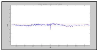
All the result shows in figure 7 for autocorrelation and figure 8, 9, 10, 11 for cross-correlation graphs for GA. By correlating a signal with itself, repetitive patterns will stand out and make it easier to see. After the process runs for a few minutes, the result produce is a perfectly sharp spike and gives impact on the system’s latency. For cross-correlation test, it is important to examine all the graph at once. To be known that the validation test is stable, all the cross-correlation graph produced should be within its confident line. Hence, GA’s validation test shows that it is stable since all the graph produce within the confident line.

Figure 7: GA’s autocorrelation test Figure 8: Cross-correlation of input and residual for GA

Figure 9: Cross-correlation of input square and residual for GA

Figure 10: Cross-correlation of input square and residual square for GA

Figure 11: Cross-correlation of residual and (input*residuals) for GA

All the result shows in figure 12 for autocorrelation and figure 13, 14, 15, 16 for cross-correlation graphs for PSO. For autocorellation test graph the result produce same goes as GA’s result. For cross-correlation test, PSO’s validation test shows that it is not so stable since there is lines that produce out of the confident line. This is because there was an existance of noise during the analysis. Hence, we can conclude that GA produce more stable graph than PSO.

Figure 12: PSO’s autocorrelation test Figure 13: Cross-correlation of input and residual for PSO

Figure 15: Cross-correlation of input square and residual square for PSO

Figure 16: Cross-correlation of residual and (input*residuals) for PSO

Conclusion

The experiment of Heat Exchanger QAD model BDT921 has been done in the Control Laboratory of UTHM. All of the 582 data from the graph of data recorder is used to find ARMAX parameters, transfer function of plant, do the validation test and compared the actual data with prediction model by GA and PSO.Between GA and PSO, we can conclude that PSO produces much better result for this analysis. Through mean square error (MSE) result, error produced by PSO is lower than GA. It is important because, the least value of error, the effective heat exchanger will be produce. However, in validation test, we can analyze that GA produce much stable graph with less noise exists.

Acknowledgement

The author would like to thanks Universiti Tun Hussein Onn Malaysia (UTHM), Johor for the equipment provided throughout the work of study and for supporting this research.

References

[1] Ibrahim, Saifudin bin Mohamed. (2005). The PID Controller Design using Genetic Algorithm. Toowoomba, Queensland: University of Southern Queensland.

[2] Ljung, Lennart. (1998). System Identification: Theory for the User. Englewood Cliffs,NJ: Pearson Education.

[3] Engelbrecht, A. P. (2006). Particle Swarm Optimization: Where does it belong? Proc, IEEE Swarm Intell,Swmp, 48-54.

[4] Eialli, Taan S. (2004). Discrete Systems and Digital Signal Processing with MATLAB. New York: CRC Press.

[5] Gupta, S. a. (2014). Robust PID Tuning of Heat Exchanger System using Swarm Optimization Method. International Journal of Recent Technology of Engineering (IJRTE), 2277-3878.