Validation Study Illustrates the Accuracy of Operational Modal Analysis Identification

(1)

International Journal of Emerging Technology and Advanced Engineering

Website: www.ijetae.com (ISSN 2250-2459, Volume 2, Issue 11, November 2012)

658

Validation Study Illustrates the Accuracy of Operational Modal

Analysis Identification

Gomaa, F.

1

, Tayel, M.

2

, Kandil, K.

3

, Hekal, G.

4 1

Assistant Professor, 4Assistant lecturer, Faculty of Engineering, Menofia University, Egypt 2_{Professor of Reinforced Concrete Structures,Faculty of Engineering, Menofia University, Egypt}

3_{Professor of Steel Structures,Faculty of Engineering, Menofia University, Egypt} Abstract— In the recent few decades, Operational Modal

Analysis OMA, also known as Output Only or Ambient Vibration Test, has become a powerful tool for a wide range of applications in the field of civil engineering. These applications include structural health monitoring, finite element model updating and structural modifications in case of presence of vibration problems. In such tests, structural modal parameters are extracted from structure responses to unknown forces. Modal parameters include resonance frequencies, mode shapes and modal damping. The current paper is concerned with comparing three different techniques used for extracting modal parameters from OMA measurements. These techniques are Frequency Domain Decomposition FDD, Enhanced Frequency Domain Decomposition EFDD and Stochastic Subspace Identification SSI. In order to achieve such aim, an output only vibration test was conducted to a small scale two storey steel frame. The experimentally obtained mode shapes were validated through calculating modal assurance criteria between each two techniques. A comparison of the frequencies obtained from experimental and numerical analysis by ABAQUS program is provided as well. The results showed that the three techniques gave almost identical results regarding to resonance frequencies and mode shapes. On the other hand, EFDD and SSI gave different values of damping ratios. SSI is a parametric technique suitable for high order modes using stable mode working in time domain, while EFDD is working in frequency domain.

Keywords— Modal assurance criteria, Modal damping, Mode shapes, Operational modal testing, Resonance frequencies

I. INTRODUCTION

Output-only modal testing is an experimental method which determines the system’s dynamic characteristics and defines a dynamic model of a structure.

Compared to classical approach, output only modal testing represents an alternative of extraordinary importance in the field of structural engineering where structures are hard to be artificially excited and there are natural sources of vibration like wind, traffic, waves...etc. i.e., instead of exciting the structure artificially and dealing with natural excitation as an unwanted noise source, the natural excitation is used as the excitation source. Real case examples on testing of some civil engineering structures can be found on [1] to [6]. The difficulty associated with output-only test is that the measured response is often noisy and contains the characteristics of the structure as well as the characteristics of the unknown excitation force. So, the art of output only modal identification is to be able to distinguish the structural modes from the operational modes. In output only modal test, structural response is captured by one or more reference sensors, at fixed positions, simultaneously with a set of roving sensors, placed at different measurement points along the structure, in different setups. The choice of measurement points on the tested structure depends on the aim of the test and the recourses available. Different identification techniques, working in either time or frequency domain, are followed to estimate modal parameters. See [6] to [10]. In the current work, the computer software ARTeMIS extractor [11] was used to perform the modal identification of the structure using both frequency domain decomposition and stochastic subspace identification techniques. The obtained results are compared and validated.

II. TESTED STRUCTURE

(2)

International Journal of Emerging Technology and Advanced Engineering

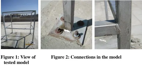
[image:2.612.347.572.124.420.2]

659 A hot rolled box section of 20 × 20 × 1.5 mm dimension was selected for both columns and girders. The beams to column connections were fully welded to make rigid connections. The columns were bolted to a rigid concrete base through 5mm thickness steel plates welded to the lower end of each column (figure 2).

Figure 1: View of Figure 2: Connections in the model tested model

III. PRELIMINARY FINITE ELEMENT ANALYSIS

In planning stage of the test, finite element analysis helps in estimation of many parameters such as sampling frequency, the desired number of measured DOFs, best location of reference sensors, data recording duration and other related issues.

Theoretical analysis was conducted by finite element method using the well known package ABAQUS/Standard Version 6.8 [12]. In this stage, natural frequencies and mode shapes of the tested model were extracted using *FREQUENCY step. The assumptions are that The structure has constant stiffness and mass effects, and there is no damping.

The structural elements were modelled using 2 node linear beam element type B31. This element has six degrees of freedom at each node: translations and rotations about x, y, and z. The connections on beam to column joints and base were assumed to be fully rigid. The material properties of the structure are listed in table 1.

Numerical bending, torsion and diagonal mode shapes and their associated natural frequencies are shown in figure 3 and table 2.

TABLE 1

MATERIAL PROPERTIES FOR FINITE ELEMENT ANALYSIS OF

STEEL FRAME MODEL

Elasticity modulus, MPa 2E5

Poisson's ratio 0.3

Mass density, N.sec2/mm4 7.849E-9

Table 2

Natural frequencies for preliminary finite element model

Mode No.

Description Natural frequency, f, Hz

1 1st bending, x direction 34.055

2 1st bending, y direction 37.042

3 1st torsion, x – y plan 45.266

4 1st diagonal, x – y plan 84.959

5 2nd bending, y direction 112.64

6 2nd_{bending, x direction} _117.23

7 2nd torsion, x – y plan 144.89

8 2nd diagonal, x – y plan 155.54 (a) Base

connection

(b) Beam to column connecti on

First bending mode x-direction f= 30.055Hz

First bending mode y-direction f= 37.042Hz

First torsion mode x-y plane f= 45.266Hz

First diagonal mode x-y plane f= 84.959Hz

Second bending mode y-direction f= 112.64Hz

Second bending mode x-direction f=117.23 Hz

Second torsion mode x-y plane f=144.89 Hz

Second diagonal mode x-y plane f= 155.54Hz

[image:2.612.50.291.213.326.2] [image:2.612.59.283.638.702.2]

(3)

International Journal of Emerging Technology and Advanced Engineering

660 IV. OUTPUT-ONLY MODAL TEST

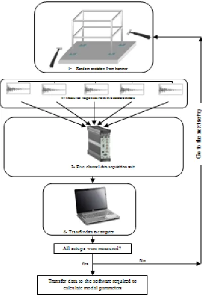
The test was conducted to the model in the Housing and Building Research Center, HBRC, in Cairo, Egypt. Randomly generated impact loads by an impact hammer were used to vibrate the model. The impacts were applied to the base slab in different directions to ensure that all modes of the model were sufficiently triggered. For acquisition of data, a five channel pulse analyzer system was used together with uni-axcial accelerometers. Based on the preliminary finite element analysis, the measurement duration was selected as 30 seconds which is long enough with respect to the Brinker criterion (1000 periods) [14].

In the test, it was aimed to get the global mode shapes and corresponding natural frequencies and modal damping ratios. To get the aimed behavior, the accelerometers were placed towards the corners of the model in two orthogonal directions as shown in figure 4.

[image:3.612.350.550.238.540.2]

Because the capacity of the data logger and number of accelerometers was limited , it was required to create a measurement sub steps using reference points. In this type of measurement setup, one or more accelerometers are kept as fixed while the other accelerometers were moved from one point to another. For this purpose, the tests on the steel building model were carried out using two sub-steps where two accelerometers were used as reference ones. The position of reference accelerometers was selected at the largest expected deformation i.e. the top floor. The measurement setups and accelerometer directions are given in Figure 4. A block diagram of the test steps is shown in figure 5.

Figure 4: Test setups

V. SAMPLES FROM MEASURED DATA

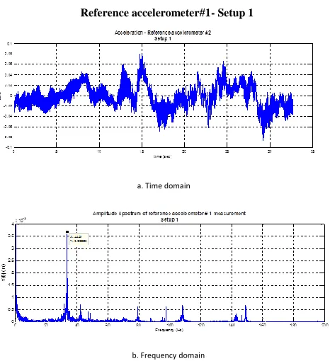
Samples from captured respnses are presented. To get more convenient outcoms, time data was transferred to frequency domain by applying Fast Fourier Transform, FFT, using MATLAB program [13]. Figures 6 and 7 show measured acceleration response and corresponding amplitude function at reference accelerometer 1 and 2 respectively. These are taken from setup 1.

It can be seen that some peaks appear at figure 5.b. Those peaks occure at the resonance frequencies of the system. Peaks in the figure appear at frequencies 33.54, 42.27, 79.16, 108.1, 143.1 and 149.1 Hz. Referring to figure 4, in this case bending modes in y direction as well as torsion and diagonal modes in x-y plane are excited. This is logic since the measured acceleration is in y direction.

Figure 5: Measurement procedure

For response data at reference accelerometer 2 for the same data set and testing case. Time response and its spectrum are shown in figure 7 a,b. In this case, the response is measured in x direction so it is clear that modes at frequencies 31.68, 42.33, 79.16, 115.1, 143.1 and 149.1 Hz are excited which are bending modes in x direction, and torsion and diagonal modes in x-y plan.

One important note is that response spectra are capable of showing the most participated modes through the amplitude values. the highest amplitudes occur at the first bending mode in y direction (curser value in figure 6.b) and

the first bending mode in x direction (curser value in figure 7.b)

Reference accelerometer 1

Reference accelerometer 2

Roving accelerometer 1

[image:3.612.38.286.493.584.2]

(4)

International Journal of Emerging Technology and Advanced Engineering

661

VI. MODAL PARAMETERS EXTRACTION TECHNIQUES

A. FREQUENCY DOMAIN DECOMPOSITION,FDD

Frequency domain decomposition is a nonparametric frequency domain technique meaning that modal parameters are estimated directly from curves. Theoretical background of FDD is published in many references including [8, 9, 14, 15 and 16].

In this technique, Discrete Fourier Transform (DFT) is performed to the raw time data to obtain acceleration spectral density matrices [Gyy(ω)] for all the series of measurements. Each element of those matrices is a spectral density matrix function. The diagonal elements of the matrix are the magnitudes of the spectral densities between a response and itself (power spectral densities). The off diagonal elements are the cross spectral densities between the different responses. All matrices are Hermitian (symmetric with complex conjugate elements around the diagonal). So, we have:

(1)

The diagonal elements are real numbers while the off diagonal elements are complex valued numbers.

The second step of analysis is performing Singular Value Decomposition, SVD on the previously obtained spectral density matrices. This step decomposes each matrix into a product of tree matrices as in equation 2





   

H

yy

G ()    

(2)

With

     

H   I ₍₃₎

Where, [Ʃ] is the singular value which is diagonal matrix and [Φ] is the singular vector unitary matrix. This matrix represents mode shapes.

The simple Peak Picking technique is applied in the first singular value line to obtain frequency and associated mode shapes. In this technique no damping ratios are estimated.

B. Enhanced Frequency Domain Decomposition, EFDD

Enhanced frequency domain decomposition is a parametric technique allowing estimates of resonance frequencies, mode shapes and modal damping ratios by computing auto and cross correlation functions. In this technique, the SDOF power spectral density function identified around a resonance peak identified by the previously explained FDD is returned to the time domain using the Inverse Discrete Fourier Transform (IDFT) to the auto spectral density functions.

[image:4.612.72.297.147.377.2]

a. Time domain

Figure 6: Measured response of structure

Reference accelerometer#1- Setup 1

b. Frequency domain

a. Time domain

b. Frequency domain

Figure 7: Measured response of structure

Reference accelerometer#2- Setup 1

q p CSD CSDpq( ) qp( ), 

* 

[image:4.612.73.306.404.659.2]

(5)

International Journal of Emerging Technology and Advanced Engineering

662 From these functions, it is straightforward to identify the modal damping ratios and obtain enhanced estimate of natural frequencies. These frequencies are evaluated looking at the time intervals between zero crossings. The modal damping ratios are estimated adjusting an exponential decay to the relative maxima of the auto correlation functions. Mode shapes are identified from the singular vectors of the spectral matrix evaluated at the identified resonance frequencies and associated with the singular values that contain the peaks. For a detailed explanation of EFDD, the reader is advised to refer to references [8, 18]

C. Stochastic Subspace Identification, SSI

SSI is a parametric method, meaning that it fits a parametric model to the time data series. While FDD operates in the frequency domain, SSI is performed directly in the time domain. the real breakthrough of SSI happened in 1996 with the publishing of the book by van Overschee and Dee Moor [22]. A more comprehensive explanation of SSI can also be found in [19, 20 and 21].

In discrete time, the system output is normally presented by the data matrix:

(4)

Where, N is the number of data points.

The Block-Henkel matrix, Yh, constructed from output signals is simply a gathering of a family of matrices that are created by shifting the data matrix.[19]

(5)

In van Overschee and Dee Moor [22], O is defined as the projection of the row space of the "future" outputs on the row space of the "past" outputs:

(6)

Then the main stochastic subspace identification theorem states that the projection O is equal to the product of the extended observability matrix Γs and state space X0:

0

X

Os ₍₇₎ Γ and X can be extracted using the SVD of matrix O:

T

USV

O

(8)

And then define the estimates of matrix Γs and X0 by:

T V S X US 2 / 1 0 2 / 1 ˆ ˆ  

 ₍₉₎

The system matrices Ad and C can be determined from the estimates of matrix Γ as:

(10)

(11)

Once the matrices are obtained, then modal analysis is started by performing an eigen value decomposition of the

system matrix Aˆd to obtain the eigenvalues λi and the eigenvectors Ψi:

 

1

ˆ __ _

i d

A 

(12)

The continuous time poles λi are found from the discrete time poles μi by:

) exp( _i

i 

 

(13)

The modal frequency ωi and modal damping ζi are computed from: i i i i i

i  i   i

    2  

1 (14)

and

2 2

i i

i  

  

(15)

2 2 i i i i     



(16)

The mode shape matrix is found from:

 

 C ₍₁₇₎

VII. ANALYSIS RESULTS

A. FREQUENCY DOMAIN DECOMPOSITION,FDD

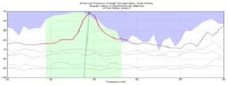
As explained earlier, frequencies and mode shape are selected from the SVD plot. when we have more than data set, the peak picking is made in an average of SVD plot of all data sets which is shown in figure 8.



y y yN



Y ₁ ₂ ...

" " " " .... .... .... .... .... .... .... 1 2 2 1 2 3 2 2 2 1 future past Y Y y y y y y y y y y Y hf hp N s s s N s N

h  

                 hp hf Y Y O ) 1 : 1 ( ) : 2

(

ˆ









s

A

d s

) 1 : 1 ( ˆ

ˆ _ _

(6)

International Journal of Emerging Technology and Advanced Engineering

663 In the figure, each peak identifies a natural frequency of the tested structure. By PP, applied to the first singular value line, 8 clear modes were identified for the tested structure. It is obvious that some peaks appear in the plot and not chosen like that one around 120 Hz, this is because the coherence function, shown in blue, at this peak is low indicating that the data at these ranges is not reliable. other peaks appear around frequencies 50, 105 and 150 Hz frequencies. these peaks are not structural peaks because, as can be seen, at these frequencies all spectral lines have peaks.

B. Enhanced Frequency Domain Decomposition, EFDD

[image:6.612.328.569.171.261.2]

The previously estimated FDD peaks are returned to time domain using IFFT in order to get more accurate estimates of frequencies and mode shapes. This also allows for damping identification from the free decay of the correlation function. figures 9 to 12 illustrate the identification of modal parameters of the third mode by EFDD. In figure 9, the identification of the SDOF Spectral Bell is performed using the FDD identified mode shape as reference vector in a correlation analysis based on a predefined Modal Assurance Criterion MAC. In this case MAC rejection level of 0.8 was used.

Figure 9: Singular value spectral bell identification from the second data set

(Third mode shape)

Figure 10 shows the IFT for the identified bell to

obtain

SDOF correlation function. as shown in figure the we have a typical response of a responding system that decays exponentially.

[image:6.612.42.289.270.348.2]

The scattered region indicates the part of the correlation function that is used for the frequency and damping estimation algorithm.

Figure 10: Normalized correlation function for the third identified mode

[image:6.612.328.562.381.453.2]

The damping is estimated by the logarithmic decrement technique from the logarithmic envelope of the correlation function. The estimation is performed by using a linear regression technique (figure11). The green curve presents the logarithm of the absolute value of all the positive and negative extremes. The red straight line is the result of the linear regression problem. The damping ratio can be found directly from the slope of this straight line.

Figure 11: Damping ratio estimation from the decay curve of the correlation function data sets

Figure 12: Natural frequency estimation from zero crossings of the normalized correlation function

[image:6.612.327.565.491.558.2]

The resonance frequency is simply obtained by counting the number of times the correlation function crosses the zero axis per second. In figure 12 they are presented as the green line. The result of the regression problem is presented as the red straight line. This regression result is based on the part of the correlation function that is inside the correlation limits shown in figure 10.

[image:6.612.52.286.535.623.2]

(7)

International Journal of Emerging Technology and Advanced Engineering

664

C. Stochastic Subspace Identification, SSI

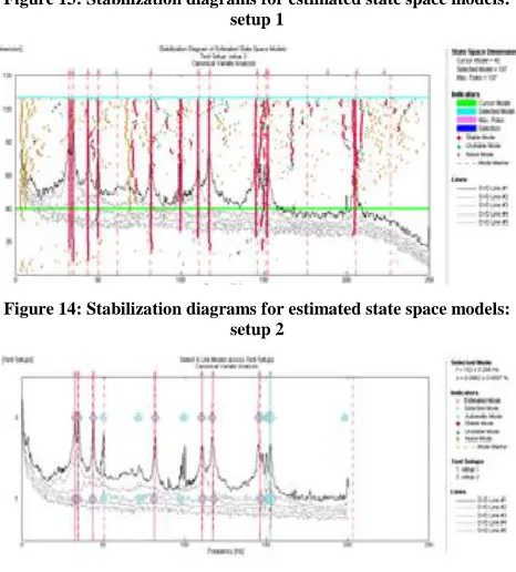
[image:7.612.53.287.245.354.2]

The stabilization diagram presents the natural frequencies of all the estimated eigenvalues as well as a background wall-paper of the Singular Value Decomposition of the spectral density matrices of the currently selected data set. This wall-paper has nothing direct to do with the estimation. However, it is a valuable help in the search of structural modes since these will be located at the spectral density peaks.

Figure 13: Stabilization diagrams for estimated state space models: setup 1

Figure 14: Stabilization diagrams for estimated state space models: setup 2

Figure 15: SSI Selected modes across the two test setups

Figures 13 and 14 show the stabilization diagram obtained by applying SSI for the two test setups. System order and stable poles can be found in these diagrams which provide modes of the structure. While figure 15 shows all selected modes across the two setups.

The experimentally identified mode shapes are shown in figure 16 and their corresponding resonance frequencies and modal damping ratios are shown in table3.

Table 3

System identified frequencies and damping ratios

Mode no.

FDD EFDD SS1

f, Hz f, Hz ζ f, Hz ζ

1 32.5 32.56 0.607 32.49 0.3339 2 34.5 34.51 0.5364 34.5 0.3211 3 43.75 43.54 0.3399 43.57 0.1496 4 81.75 81.43 0.1942 81.47 0.1696 5 110.8 110.6 0.2378 110.4 0.2752 6 116.8 117.1 0.2467 117.2 0.2826 7 145.3 145.8 0.2425 145.8 0.2789 8 152.5 152.5 0.1151 152.5 0.096

Figure 16: Experimentally identified mode shapes Figure 15:

Experimental mode shapes

Mode 1 Mode 2 Mode 3 Mode 4

[image:7.612.52.285.368.626.2]

(8)

International Journal of Emerging Technology and Advanced Engineering

665 VIII. VALIDATION OF TEST RESULTS

once the modal parameters are calculated, there are many tools for validation are applied to them. In the current paper, both modal assurance criteria and comparison with Finite element analysis results are presented.

A. Modal Assurance Criteria

A widely used technique for comparing mode shapes is the Modal Assurance Criterion (MAC). It gives quantitatively a good idea of the closeness between two families of mode shapes ϕ (1) and ϕ (2):[23]

(18)

In this equation, the MAC is computed between mode i of the first family and mode j of the second family. MAC values oscillate between 0, representing no consistence correspondence, and 1, representing a perfect correlation. In practice, a value greater to 0.9 is commonly recognized as acceptable to establish the correspondence between two mode shapes.

It is recommended that modal parameters are estimated using different techniques and their shapes compared using Cross MAC calculations [8]. If different techniques yield similar results it is very likely that a physical mode shape is found.

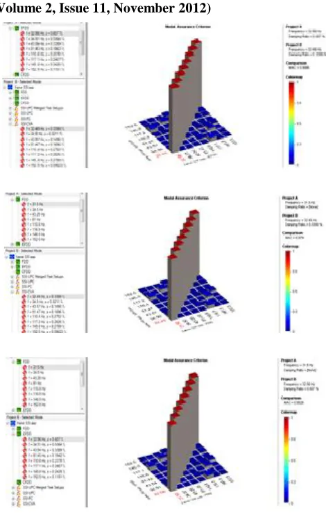
[image:8.612.325.560.119.488.2]

For the tested frame, MAC matrices between FDD-EFDD, FDD-SSI and between EFDD -SSI are shown in figure 17:

Figure 17: Experimentally identified mode shapes



{ } { }



{ } { }



} { } { )

,

( ₍₁₎ ₍₁₎ ₍₂₎ ₍₂₎

2 ) 2 ( ) 1 ( )

2 ( ) 1 (

j T j i T i

j T i j

i

MAC

   

  

(9)

International Journal of Emerging Technology and Advanced Engineering

666 As shown from figure 17, the agreement between mode shapes obtained with the three methods leads to diagonal values in the MAC matrices varying from 97.9% to 100%, indicating a high level of correlation between the three sets of mode shapes. The maximum coupling value (5.8%) occurs between the first and sixth modes which are the first and second bending modes in x- direction. Also a coupling value of about (4.2% ) occurs between the third and seventh modes which are first and second torsion modes. All the other coupling indicates are below (2%). The MAC matrices calculated between the three sets of mode shapes indicated that the best correlation was found between EFDD and SSI. In this case, values are varying between 99.4% to 100%. This demonstrates the effectiveness of these two techniques in identifying modal parameters.

B. Comparison with finite element analysis

Results of a finite element analysis of the system under test can provide another method of validating the modal model. The comparison presented here is made between experimental and numerical frequencies. It is illustrated in many references that the acceptable difference margin between analytical and experimental results is 10%.

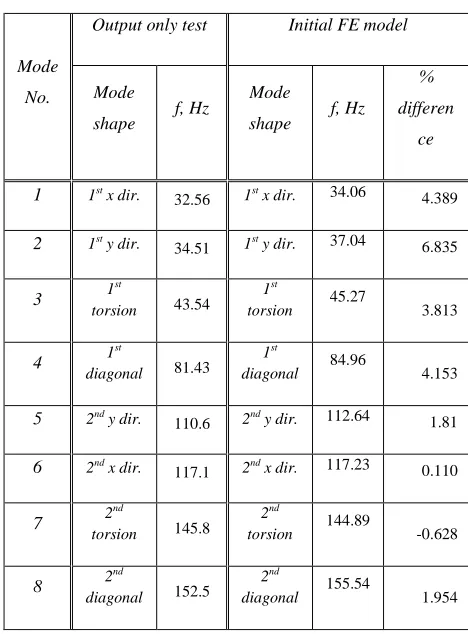
Recalling the natural frequencies obtained by initial Finite Element model, table 4 shows a comparison between numerical and EFDD modal frequencies for the tested frame. It is obvious that the order of all the mode shapes was as predicted by the experimental tests shown in figure 1, and natural frequency difference between test and analysis is within the accepted 10% margin.

IX. DISCUSSION AND CONCLUSIONS

The paper presented an output only modal test on a steel frame. A preliminary finite element analysis was performed to be used as a key tool in planning stage of the test. Data obtained was analyzed using ARTeMIS software. Three techniques were used for modal parameter extraction. These techniques are FDD, EFDD, SSI. Modal assurance criteria MAC were obtained as a validation tool for experimental data. experimental frequencies were compared to analytical ones as well.

Based on the above work it can be concluded that:

[image:9.612.335.569.202.519.2]

1.

The

output-only vibration testing provides an accurate estimate of modal parameters in both time and frequency domains. A good agreement in identified natural frequencies has been found with frequency domain decomposition FDD based on peak picking method and the time domain based stochastic subspace identification SSI.

Table 4

Frequency comparison between output only test and initial FE

model results

Mode

No.

Output only test Initial FE model

Mode

shape f, Hz

Mode

shape f, Hz

%

differen

ce

1 1st_{x dir.}

32.56 1st x dir. 34.06 4.389

2 1st_{y dir.}

34.51 1st y dir. 37.04 6.835

3 1

st

torsion 43.54 1st

torsion 45.27 3.813

4 1

st

diagonal 81.43 1st

diagonal 84.96 4.153

5 2nd_{y dir.}

110.6 2nd y dir. 112.64 1.81

6 2nd_{x dir.}

117.1 2nd x dir. 117.23 0.110

7 2

nd

torsion 145.8 2nd

torsion 144.89 -0.628

8 2

nd

diagonal 152.5 2nd

(10)

International Journal of Emerging Technology and Advanced Engineering

667 The resonance frequencies obtained by both methods

are almost identical as the maximum difference in values didn't exceed 0.4%. Additionally, the mode shapes comparison using MAC values showed that the diagonal values in the MAC matrices are varying from 97.9% to 100%, indicating a high level of correlation between the three sets of mode shapes.

2. In the Frequency Domain Decomposition (FDD) , the simple peak picking technique gives frequency and mode shape at the selected frequency, whereas the Enhanced FDD (EFDD) method adds estimation of damping as well and the estimates of frequency and mode shape are improved by fitting a SDOF model to the singular values in a user-defined frequency band around the peak.

3. The modal damping estimated by EFDD technique is almost twice those estimated by SSI for the first four mode shapes. It can be noted that damping values by EFDD are closer to the common values recommended for steel structures. This difference may happened because SSI is more suitable for high order modes which is not the case in this study where the frequency range is 0-200 Hz.

REFERENCES

[1] Baptisca, M., Mendes, P., COSTA, A., Sousa, C., Afilhado, A. and Silva, P.2004 Use of ambient vibration testing for modal evaluation of a 16 floor reinforced concrete building in Lisbon, Portugal. 13th World Conference on Earthquake Engineering Vancouver, B.C. Canada, August 1- 6, 2004 Paper No. 1985.

[2] El- Borgi, Smaoui, S., Cherif, F., Bahlous, S. and Ghrairi, A.2004 Modal identification and finite element model updating of a reinforced concrete bridge. Emirates Journal for Engineering Research, 9 (2), 29-34.

[3] Garziera R, Amabili M and Collini L. 2007 Structural health monitoring techniques for historical buildings. 4th conference of END, Buenos Aires.

[4] Lamarche1, C., Paultre, P., Proulx1, J. and Mousseau, S. 2008 Assessment of the frequency domain decomposition technique by forced-vibration tests of a full scale structure. Earthquake Engineering and Structural Dynamics. 37: 487- 494

[5] Tashkov, L., Krstevska, L., Garevski, M. and Gocevski, V. 2008 Experimental investigation of seismic stability on masonry walls at Beauharnois powerhouse. The 14th World Conference on Earthquake Engineering October 12-17. Beijing.

[6] Cunha, E. and Caetano, A. 2005 Experimental modal analysis of civil engineering structure.. First international modal analysis conference, IOMAC, Copenhagen, Denmark.

[7] Le, T. and Tamura Y. 2009 Modal identification of ambient vibration structure using frequency domain decomposition and wavelet transform”. The Seventh Asia-Pacific Conference on Wind Engineering, November 8-12. Taipei, Taiwan.

[8] Gade, S., Moller, N., Herlufsen, H. and Hansen, H. 2006 Frequency domain techniques for operational modal analysis. IMAC- XXIV, January. A Conference and Exposition on Structural Dynamics. [9] Gade, S., Moller, N. and Herlufsen, H. 2006 Identification

techniques for operational modal analysis - An overview and practical experiences. IMAC- XXIV. January, 30. A Conference and Exposition on Structural Dynamics.

[10] Yousaf, E. 2007 Output only modal analysis. Master thesis. Mechanical Engineering Department, Bleking Institute of Technology, Karlskrona, Sweden.

[11] Structural Vibration Solutions ApS. 2011 ARTeMIS Extractor, User’s Manual, Denmark.

[12] ABAQUS PROGRAM, USERS AND MANUAL, 6.8. 2008 [13] MATLAB Version 7.10.0.499 (R2010a). The Mathworks, Inc. [14] Brincker, R, Ventura, C. and Anderson P. 2003 Why output-only

modal testing is a desirable tool for a wide range of practical applications. 21st International Modal Analysis Conference IMAC, Kissimmee, Florida

[15] Batel, M. 2002 Operational modal analysis- another way of doing modal testing. Sound and vibration.

[16] Brincker, R., Zhang, L. and Andersen, P. 2001 Modal identification of output-only systems using frequency domain decomposition. Institute of Physics Publishing, Smart materials and structures, 10, 441-445.

[17] Brincker, R., Zhang, L. and Andersen, P. 2000 Modal identification from ambient responses using frequency domain decomposition”; International Modal Analysis Conference (IMAC), San Antonio, Texas.

[18] Brincker, R., Zhang, L. and Andersen, P. 2001 Damping estimation by frequency domain decomposition. Proceedings of SPIE, Society of Photo-Optical Instrumentation Engineers, Bellingham. Vol. 4359 (1), pp. 698-703.

[19] Brincker, R. and Andersen, P. 2006 Understanding stochastic subspace identification. Proceedings of the 24th International Modal Analysis Conference (IMAC), St. Louis, Missouri.

[20] Tanaka, H., Mutawa, J. and Katayama, T. 2005 Stochastic subspace identification of linear systems with observation outliers. Proceedings of the 44th IEEE conference on Decision and Control, and the European Control Conference 2005, Seville, Spain. [21] Jiravacharadet, M. 2008 Stochasic subspace system identification of

a multi storey building. Suranaree J. Sci. Technol. 15(4):287-291. [22] Overschee, P. and Moor, B. Subspace identification for linear

systems. Kluwer Academic Publisher.

[23] Allemang, R. 2003 The modal assurance criterion- twenty years of use and upuse. Sound and Vibration. pp. 14-21.