Shortest Path Position Estimation between Source and Destination nodes in Wireless Sensor Networks with Low Cost.

(1)

International Journal of Emerging Technology and Advanced Engineering

Website: www.ijetae.com (ISSN 2250-2459, Volume 2, Issue 4, April 2012)

6

Shortest Path Position Estimation between Source and

Destination nodes in Wireless Sensor Networks with Low Cost.

N. Pushpalatha

1

, Dr.B.Anuradha

2

,

1_{Assistant Professor, Department of ECE, AITS, Tirupathi}

2_{Associate Professor, Department of ECE,S.V. University College of Engineering, Tirupathi.}

1

[email protected] 2_{[email protected]}

Abstract - A sensor network comprised of sensing (measuring), computing, and communication elements that gives an administrator the ability to instrument, observe, and react to events and phenomena in a specified environment. The administrator typically is a civil, governmental, commercial, or industrial entity. The environment can be the physical world, a biological system, or an information technology framework. Network sensor systems are seen by observers as an important technology that will experience major deployment in the next few years for a plethora of applications, not the least being national security. Typical applications include, but are not limited to, data collection, monitoring, surveillance, and medical telemetry. In addition to sensing, one is often also interested in control and activation. There are four basic components in a sensor network: (1) an assembly of distributed or localized sensors; (2) an interconnecting network (usually, but not always, wireless-based); (3) a central point of information clustering; and (4) a set of computing resources at the central point (or beyond) to handle data correlation, event trending, status querying, and data mining. In this paper, the sensing and computation nodes are considered part of the sensor network; in fact, some of the computing may be done in the network itself. In the MATLAB simulation, a random network of 50 nodes was created and Dijkstra's algorithm was used to find the routes between anchors [4]. This paper proposes a Dijkstra’s algorithm which uses the connectivity of information, the estimated distance information among the sensor nodes and find out the Shortest Path Position Estimation between Source and Destination nodes in Wireless Sensor Networks with Low Cost.

Key words- Dijkstra’s algorithm, Wireless Sensor Networks, Shortest path, Low cost

I. I

NTRODUCTION

Wireless Sensor Networks (WSNs) are a research topic of growing interest over the recent years due to its wide applications. WSNs are a set of wireless embedded devices that have the capability of processing and communicating video and audio streams collected from the environment in a distributed fashion[1]. WSNs find applications in surveillance systems against crime and terrorist attacks. They can also be used for traffic monitoring in cities and highways. They are also very useful in military applications to locate the targets of interest (such as enemy soldiers, tanks) in the battlefield. For most WSN applications, it is important to have the knowledge of the location of the nodes in order to understand the data received. Therefore, there is a great need to develop a sensor node multidimensional scaling algorithm which can be computational resources [2]. This paper proposes a Dijkstra’s algorithm using the network connectivity information and the estimated distance information among the sensor nodes and find out the shortest path between the source node and destination node with low cost. Based on the multidimensional scaling (MDS) technique [3, 6] we derive node locations to fit the roughly estimated distances between pairs of nodes. It uses the Shortest Path Position Estimation between Source and Destination nodes in Wireless Sensor Networks with Low Cost.

(2)

International Journal of Emerging Technology and Advanced Engineering

7

Given the inter-node distances, techniques like multilateration can be used to locate the nodes [8]. Range-free techniques have also been used widely. Hop number is used as an indication of the distance to the beacon nodes in some applications [7]. However, most of the literature is on localization of traditional wireless sensor networks and not much has been discussed on shortest path between source node and destination node in wireless sensor networks, which have more sensing modalities than traditional ones.

The focus of the paper is Shortest Path Position Estimation between Source and Destination nodes in Wireless Sensor Networks with Low Cost. The paper is organized as follows. Section 2 presents the previous work of localization problem in wireless sensor networks. Proposed method has been discussed in section 3. In section 4 the problem localization in wireless sensor networks. In section 5 Simulation Results of the paper has been discussed. In section 6 Conclusion and Future work, where the future challenges and directions to improve localization in WSN technology are described.

II.

P

REVIOUSWORK

The multidimensional scaling technique, which is a technique that has been successfully used to capture the intercorrelation of high dimensional data at low dimension in social science, is used [1]. A Square method is used to estimate all sensors’ relative locations by applying MDS to compute the relative positions of sensors with high error tolerance. In order to collect some of pair wise distances among sensors, we select a number of source sensors, and they initialize the whole network to estimate some of the pair. The multidimensional scaling (MDS), a technique widely used for the analysis of dissimilarity of data on a set of objects, can discover the spatial structures in the data. It is used it as a data-analytic approach to discover the dimensions that underlie the judgments of distance and model data in a geometric space. The main advantage in using the MDS for position estimation is that it can always generates relatively high accurate position estimation even based on limited and error-prone distance information. There are several varieties of MDS. On classical MDS and the iterative optimization of MDS, the basic idea of which is to assume that the dissimilarity of data are distances and then deduce their coordinates. More details about comprehensive and intuitive explanation of MDS are available in [1-4].

In Fig.1 and Fig.2 the position estimation method and the coverage area are compared in [2]. The work presented in the paper is Distribution of nodes on square

method for wireless sensor networks by using

multidimensional scaling algorithm for position estimation. Some challenges of position estimation problem in real applications are dealt in this paper.

The conditions that most existing sensor positioning methods fail to perform well are the anisotropic topology of the sensor networks and complex terrain where the sensor

networks are deployed. Moreover, cumulative

measurement error is a constant problem of some existing sensor positioning methods [1&2]. This proposed method ables to position the sensors on a square area and also estimates the shortest path between source and destination nodes in WSNs with low cost.

0 2 4 6 8 10

Fig.1. Randomly distributed sensors in a triangulation method

0 2 4 6 8 10

(3)

International Journal of Emerging Technology and Advanced Engineering

8

III. P

ROPOSED

M

ETHOD

The Shortest path method is used to estimate all sensors’ relative locations by applying Dijkstra’s algorithm to compute the relative positions of sensors with low cost and high error tolerance. The routing algorithm is stored in the router's memory. The routing algorithm is a major factor in the performance of position estimation and distance measurement in the senor field. The purpose of the routing algorithm is to make decisions for the router concerning the best paths for estimating the positions of anchors. The router uses the routing algorithm to compute the path that would best serve to find out the shortest path between the source and destination.

3.1. Dijkstra’s algorithm

The router builds a graph of the network. Then it identifies source and destination nodes, for example R1 and R2. The router builds then a matrix, called the "adjacency matrix." In the adjacent matrix, a coordinate indicates weight. [i, j], for example, is the weight of a link between nodes Ri and Rj. If there is no direct link between Ri and Rj,

this weight is identified as "infinity."

Procedure for finding the shortest path using Dijkstra’s algorithm is as follows:

1. The router then builds a status record for each node on the network. The record contains the following fields:

 Predecessor field - shows the previous node.

 Length field - shows the sum of the weights from the source to that node.

 Label field - shows the status of node; each node have one status mode: "permanent" or "tentative."

2. In the next step, the router initializes the parameters of the status record (for all nodes) and sets their label to "tentative" and their length to "infinity".

3. During this step, the router sets a T-node. If R1 is to be the source T-node, for example, the router changes R1's label to "permanent." Once a label is changed to "permanent," it never changes again.

4. The router updates the status record for all tentative nodes that are directly linked to the source T-node. 5. The router goes over all of the tentative nodes and

chooses the one whose weight to R1 is lowest. That node is then the destination T-node.

6. If the new T-node is not R2 (the intended destination), the router goes back to step 5.

7.

If this node is R2, the router extracts its previous node from the status record and does this until it arrives at R1. This list of nodes shows the best route from R1 to R2 as shown in Fig.3

Fig.3 Flow Chart to find shortest path using Dijkstra’s algorithm

IV. P

ROBLEM

L

OCALIZATION

I

N

W

IRELESS

S

ENSOR

N

ETWORKS

(4)

International Journal of Emerging Technology and Advanced Engineering

9

The main advantage in using the Dijkstra’s for position estimation is that it can always generates relatively high accurate position estimation even based on limited and error-prone distance information. It is also one of the methods in MDS algorithms. There are several varieties of routing algorithms to find out the shortest path between the source node and destination node for position estimation, the basic idea of which is to assume that the dissimilarity of data are distances and then deduce their coordinates.

More details about comprehensive and intuitive

explanation of MDS are available in [1 & 2]. Inspired by the above multidimensional scaling techniques, present a multivariate optimization based iterative algorithm for sensor location calculation is presented in this paper. T = [tij]n×2 denotes the true locations of the set of n sensor nodes in 2-dimensional space. dij(T) stands for the distance between sensor i and j based on their position in T and such as type (1)

 

2

1

1 2 ( ) m

ia a

ij ja

d x

t



 

 

 _





_ (1)

The collected distance between node i and j is δij . If the

errors are ignored in distance measurement, δij is equal to

dij (T ). We will discuss the error effects to location

estimation caused by differences between δij and dij (T )

later. If only a portion of pair wise distances are collected, some δij are undefined for some i, j. In order to assist

computation, define weights wij with value1 if δij is known

and 0 if δij is unknown and assume as in the following

induction.

 

ij

d T

ij





(2)

X=[xij]n×2 denotes the estimated locations of the set of n

sensor nodes in 2-D space. X randomly initialized as X[0]and will be updated into X[1] ,X[2],X[3] ….to approximate T with iterative algorithm.dij(X) is the

calculated distance between sensor i and j based on their estimated position X and as

 

2

1

1 2

( )

m ia a

ij ja

d

x



 

 

 _





_ (3) (3)

To find a position matrix X to approximate T by minimizing as

 

ij

(

_ij

 

ij

)

2 i j

x

w d x













(4) (4)

This is a quadratic function without constraints. The minimum value of such functions is reached when its gradient is equal to 0. The MDS algorithm to estimate the positioning of sensors is as given below.

 Compute the matrix of squared distance D2, where

D = [dij ]n×n;

 Compute the matrix J with J = I−e∗(eT)/n, where e = (1, 1, . . . , 1);

 Apply double centering to this matrix with H=

−½JD2J ;

 Compute the Eigen- decomposition H=UVUT

 To get the i dimensions of the solution (i=2 in 2-D case), it is denoted that the matrix of largest i Eigen values by Vi and Ui the first i columns of U.

The coordinate matrix of classical scaling is X=UiVi1/ 2.

In many situations, the distances between some pairs of sensors in the local area are not available. When this happens, the Dijkstra’s algorithm employed to compute the relative coordinates of adjacent sensors. The є is an empirical threshold based on accuracy requirement. It is usually set it as 4% of the average radio range. This algorithm generates the relative positions of sensor nodes in X[k] .

V. S

IMULATION

R

ESULTS

(5)

International Journal of Emerging Technology and Advanced Engineering

10

0 100 200 300 400 500 600 700 800 900 1000

1 2

3 4

5 6

7

8 ₉

10

11

12

13

14 15

16

17 18 19

20 21

22

23

24

25 26

27

28 29

30 31

32

33

34

35 36

37 38

39

40

41

42

43

44

45 46

47 48

49 50

Fig.4. Shortest path between Source node and destination node

VI. C

ONCLUSIONS

A

ND

F

UTURE

W

ORK

It is shown that the proposed algorithm works well for near uniform radio propagation. However, in the real world, radio propagation indoors and in cluttered circumstances is far from uniform. Local distance estimation may also be poor. Further simulations will be needed to determine reducing the range errors by using MDS algorithms can be to such errors. As Dijkstra’s algorithm builds the local positions and routings of the estimated sensors for applications that require absolute coordinates of nodes, waiting until large number sensor nodes has formed before transforming to absolute coordinates may be a poor choice. Using the method described here, Position estimation using the shortest path method between source node and destination node with low cost in wireless sensor networks that compute absolutecoordinates of individual nodes or sub networks independently can be developed.

(6)

International Journal of Emerging Technology and Advanced Engineering

11

Reference points are used in a 2-dimensional square computation. Additionally, simulations show that cooperative ranging, a Dijkstra’s algorithms, is capable of producing position estimates with 4% ranging error.

[image:6.595.67.535.212.525.2]

It is the best algorithm to find out Shortest path position estimation method in wireless sensor networks.

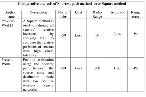
Table 1

Comparative analysis of Shortest path method over Square method

Author

name

Description

No. of

nodes

Cost

Radio

Range

Accuracy

Range

error

Work[1]

A Square method is

used to estimate all

sensors’

relative

locations

by

applying MDS to

compute the relative

positions of sensors

with

high

error-tolerance.

>50

Less

50 Low

5%

Present

Work

Position estimation

using the shortest

path between the

source node and

destination

node

with low cost in

wireless

sensor

networks

>50

Less

200 High

4%

REFERENCES

[1 ] N. Pushpalatha and Dr.B.Anuradha, “Distribution of Nodes on Square Method for Wireless Sensor Networks”, in International Journal of Computer Science and Telecommunications [Volume 3, Issue 1, January 2012].

[2 ] N.Pushpalatha and Dr.B.Anuradha, “ Study of Various Methods of Wireless Ad-hoc Sensor Networks using Multidimensional Scaling for Position Estimation” Global Journal Engineering and AppliedSciences-ISSN2249-2631(online): 2249-2623(Print) GJEAS Vol.1(3) , 2011

[3 ] Rohit Kadam, Sijian Zhang, Qizhi wang, Weihua Sheng, ltidimensional Scaling Based Location Calibration for Wireless Multimedia Sensor Networks” The 2010 IEEE/RSJ International Conference on Intelligent Robots and Systems October 18-22, 2010, Taipei, Taiwan

[4 ] X. Nguyen, M.I. Jordan, and B. Sinopli. “A kernel-based learning approach to ad- hoc Sensor network localization”. ACM Transactions on Sensor Networks, 1(1):134–152, 2005.

[5 ] XiangiJi, and HongyuanZha, “Sensor positioning in wireless Ad-hoc sensor Networks using multidimensional Scaling”, in 23rd annual joint conference of the IEEE computer and communication society, pp: 2652-2661, 2004

[6 ] F.Zhao and L.Guibas.“Wireless Sensor Networks: An Information Processing Approach”. Elsevier and Morgan Kaufmann Publishers, 2004.

[7 ] R. L. Moses, D. Krishnamurthy, and R. Patterson. “A self-localization method for wireless sensor networks”. Paper on Applied Signal Processing, 2003(4):148-158, March 2003. [8 ] Shang.Y.; Ruml.W; Zhang,Y.; Fromherz, M.P.J.” Localization

from mere connectivity”. Fourth International ACM Symposium on Mobile Ad Hoc Networking and Computing ; 2003 June 1-3; Annapolis; MD. NY: ACM; 2003; 201-212.

(7)

International Journal of Emerging Technology and Advanced Engineering

12

N . Pushpalatha completed her B.Tech at JNTU, Hyderabad and M.Tech at A.I.T.S., Rajampet. Presently she is working as Assistant Professor of ECE, Annamacharya Institute of Technology and Sciences Tirupati since 2006. She has guided many B.Tech projects. Her Research area includes Data Communications and Ad-hoc Wireless Sensor Networks.

Dr. B. Anuradha is working as Associate Professor of ECE, at Sri Venkateswara University

College of Engineering since 1992. She has guided many B.Tech and M.Tech projects. At present Five Scholars are working for PhD. She has published a good number of papers in journals