Representation of spatial and temporal variability in large domain hydrological models: case study for a mesoscale pre Alpine basin

www.hydrol-earth-syst-sci.net/20/2207/2016/ doi:10.5194/hess-20-2207-2016

© Author(s) 2016. CC Attribution 3.0 License.

Representation of spatial and temporal variability in large-domain

hydrological models: case study for a mesoscale pre-Alpine basin

Lieke Melsen1, Adriaan Teuling1, Paul Torfs1, Massimiliano Zappa2, Naoki Mizukami3, Martyn Clark3, and Remko Uijlenhoet1

1_{Hydrology and Quantitative Water Management Group, Wageningen University, Wageningen, the Netherlands} 2_{Swiss Federal Research Institute (WSL), Birmensdorf, Switzerland}

3_{National Center for Atmospheric Research (NCAR), Boulder, CO, USA}

Correspondence to:Lieke Melsen ([email protected])

Received: 10 December 2015 – Published in Hydrol. Earth Syst. Sci. Discuss.: 27 January 2016 Revised: 25 May 2016 – Accepted: 25 May 2016 – Published: 8 June 2016

Abstract.The transfer of parameter sets over different tem-poral and spatial resolutions is common practice in many large-domain hydrological modelling studies. The degree to which parameters are transferable across temporal and spa-tial resolutions is an indicator of how well spaspa-tial and tem-poral variability is represented in the models. A large de-gree of transferability may well indicate a poor representa-tion of such variability in the employed models. To inves-tigate parameter transferability over resolution in time and space we have set up a study in which the Variable Infiltra-tion Capacity (VIC) model for the Thur basin in Switzerland was run with four different spatial resolutions (1 km×1 km, 5 km×5 km, 10 km×10 km, lumped) and evaluated for three relevant temporal resolutions (hour, day, month), both applied with uniform and distributed forcing. The model was run 3150 times using the Hierarchical Latin Hypercube Sam-ple and the best 1 % of the runs was selected as behavioural. The overlap in behavioural sets for different spatial and tem-poral resolutions was used as an indicator of parameter trans-ferability. A key result from this study is that the overlap in parameter sets for different spatial resolutions was much larger than for different temporal resolutions, also when the forcing was applied in a distributed fashion. This result sug-gests that it is easier to transfer parameters across different spatial resolutions than across different temporal resolutions. However, the result also indicates a substantial underestima-tion in the spatial variability represented in the hydrological simulations, suggesting that the high spatial transferability may occur because the current generation of large-domain

models has an inadequate representation of spatial variabil-ity and hydrologic connectivvariabil-ity. The results presented in this paper provide a strong motivation to further investigate and substantially improve the representation of spatial and tem-poral variability in large-domain hydrological models.

1 Introduction

Because the parameters in hydrological models often rep-resent a different spatial scale than the observation scale, or because conceptual parameters have no directly measurable physical meaning, calibration of hydrological models is al-most always inevitable (Beven, 2012). The increased com-plexity of hydrological models and the increased application domain has resulted in more complex and time consuming optimization procedures for the model parameters. However, although recent developments in e.g. satellites and remote sensing can provide spatially distributed data to construct and force models, discharge measurements are still required to calibrate and validate model output.

Both to decrease calculation time of the optimization pro-cedure and to be able to apply the model in ungauged or poorly gauged basins and areas, many studies have fo-cused on the transferability of parameter values over time, space, and spatial and temporal resolution (e.g. Wagener and Wheater, 2006; Duan et al., 2006; Troy et al., 2008; Samaniego et al., 2010; Rosero et al., 2010; Kumar et al., 2013; Bennett et al., 2016). Sometimes it is assumed that pa-rameters are directly transferable, for example by calibrating on a coarser time step than the time step at which the model output will eventually be analysed (e.g. Liu et al., 2013; Costa-Cabral et al., 2013). Troy et al. (2008) rightly question what the effect is of calibrating at one time step and transfer-ring the parameters to another time step. Their results suggest that the time step had only limited impact on the calibrated parameters and thus on the monthly runoff ratio. On the other hand, Haddeland et al. (2006) found that modelled moisture fluxes are sensitive to the model time step. Several studies (e.g. Littlewood and Croke, 2008, 2013; Kavetski et al., 2011 and Wang et al., 2009) have found that parameter values are closely related to the employed time step of the model. Chaney et al. (2015) investigated to what extent monthly runoff observations could reduce the uncertainty around the flow duration curve of daily modelled runoff. They found a decrease in the uncertainty around the flow duration curve when the monthly discharge observations were used, but the magnitude of the reduction was dependent on climate type. Recently, Ficchì et al. (2016) conducted a thorough analysis of the effect of temporal resolution on the projection of flood events, where it was shown that the flood characteristics de-termined the sensitivity for the temporal resolution.

Less intuitive and less common is to transfer parameters across different grid resolutions. Haddeland et al. (2002) showed that the output of the Variable Infiltration Capacity (VIC) model was significantly different when the parame-ters of the model were kept constant for several spatial res-olutions. For the same model, Liang et al. (2004) showed that model parameters calibrated at a coarse grid resolution could be applied to finer resolutions to obtain comparable results. Troy et al. (2008), on the contrary, found that cali-brating the VIC model on a coarse resolution significantly affected the model performance when applied to finer resolu-tions. Finnerty et al. (1997) investigated parameter

transfer-ability over both space and time for the Sacramento model, and showed that it can lead to considerable volume errors.

Although the ambition of GHMs is to move towards hyper-resolution (∼1 km and higher), more physically based catch-ment models have already been applied at spatial resolutions of the order of 100 m. Also for these models at this scale, the effect of spatial resolution has been investigated (e.g. Vivoni et al., 2005; Sulis et al., 2011; Shrestha et al., 2015). Even for fully coupled surface-groundwater land-surface models, the effect of spatial resolution on hydrologic fluxes was found to be considerable (Shrestha et al., 2015).

The impact of transferring parameters across spatial and/or temporal resolutions on model performance is thus ambigu-ous, but relevant in the light of hydrological model develop-ment, especially for GHMs which are at the upper bound-ary of computational power and data availability. Calibration on a coarse temporal or spatial resolution and subsequently transferring to a higher resolution could potentially reduce computation time, and it is therefore relevant to investigate the opportunities. But parameter transferability across spatial and temporal resolutions is also interesting for another rea-son: it is an indicator of the degree to which spatial variability and temporal variability are represented in the model. Ideally, in a model that describes all relevant hydrological processes correctly, parameters should to a large extent be transferable over time because longer time steps are simply an integra-tion of the shorter time steps. On the other hand, parameters should not be or be hardly transferable over space, because the physical characteristics which they represent are different from place to place. Investigating parameter transferability across spatial and temporal resolutions can thus provide in-sight into the model’s representation of spatial and temporal variability.

In this study, we employ the Variable Infiltration Capac-ity (VIC) model (Liang et al., 1994), which has also been applied at the global scale (Nijssen et al., 2001; Bierkens et al., 2014), to study parameter transferability across tempo-ral and spatial resolutions, accounting for the difference be-tween uniform and distributed forcing. We applied this study to a well-gauged meso-scale catchment in Switzerland (the Thur basin, 1703 km2) on spatial resolutions that are relevant for hyper-resolution studies (1 km×1 km, 5 km×5 km and 10 km×10 km, as well as a lumped model which represents the 0.5◦grid used in many global studies). We use the most common temporal resolutions for which discharge data are available (hourly, daily, monthly). We ran the models both with distributed forcing (different forcing input for each grid cell) and with uniform forcing (same forcing input for each grid cell), where the latter is in line with many of the data sets currently used for forcing global hydrological models (e.g. WATCH forcing data, 0.5◦).

500 m 1000 m 1500 m 2000 m

Discharge (m

3s

−1

)

2002/2003

A S O N D J F M A M J J A S 100

300 500 700 900

2002/2003

A S O N D J F M A M J J A S 100

300 500

2002/2003

A S O N D J F M A M J J A S 50

100

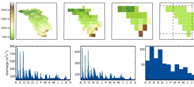
Figure 1.Overview of the spatial and temporal resolutions employed in this study. Top panels from left to right: DEM (digital elevation

model) grid cells for 1 km×1 km, 5 km×5 km, 10 km×10 km resolution and the lumped model. The circle in the left panel shows the

location of the Thur outlet where the discharge is measured. The dotted lines in the right panel indicate a 0.5◦grid. Bottom panels: the three

temporal resolutions; observed discharge at an hourly, daily and monthly time step.

probabilistic approach rather than a deterministic approach: essentially we employ a GLUE-based approach (Beven and Binley, 1992, 2014) in which we implicitly account for pa-rameter uncertainty. We quantify papa-rameter transferability by evaluating the overlap in behavioural sets for different tem-poral and spatial resolutions. To determine the behavioural sets, we make use of three different objective functions fo-cusing on high flows, average conditions, and low flows. It is also novel that we test the effect of forcing on the results, and that we use several subbasins to explain the results. Our case study provides a benchmark for parameter transferability for models applied at larger scales, dealing with the same spatial and temporal resolutions as employed here. The results of our study also provide an indication of the current status of spatial and temporal representation in the VIC model, being representative of a larger group of land-surface models.

2 Catchment and data description 2.1 Thur basin

The Thur basin (1703 km2; see Figs. 1 and 2) in north-eastern Switzerland was chosen as the study area, because of the ex-cellent data availability in this area and because of its rel-evance as a tributary of the river Rhine (Hurkmans et al., 2008). The main river in the basin (the Thur) has a length of 127 km. The average elevation of the basin is 765 m a.s.l., and the mean slope is 7.9◦_{(based on a 200 m×200 m}

resolu-tion DEM and slope file). The basin outlet is situated at An-delfingen at an elevation of 356 m a.s.l. (Gurtz et al., 1999). The basin has an Alpine/pre-Alpine climatic regime, with high temperature variations both in space and time (Fig. 3). Precipitation varies from 2500 mm yr−1 in the mountains to 1000 mm yr−1 in the lower areas. Part of the year the basin is covered with snow. The most striking feature in the

Halden

StGallen Herisau

Appenzell

Mogelsberg Rietholzbach

Jonschwil Wängi

Frauenfeld

Andelfingen (Thur outlet)

0 5 10 20 Kilometers

47.597N,8.681E

.

Figure 2.The Thur basin and the nine sub-basins for which

dis-charge data were available.

Thur basin is the Säntis, an Alpine peak with an altitude of 2502 m. The dominant land use in the Thur basin is pasture. Within the Thur basin, measurements for nine (nested) sub-catchments are available (see Fig. 2). The smallest gauged sub-catchment is the Rietholzbach catchment (3.3 km2; see Seneviratne et al., 2012); the largest is Halden (1085 km2). Both the Rietholzbach and the Thur have been the subject of many previous studies (e.g. Gurtz et al., 1999, 2003; Jasper et al., 2004; Abbaspour et al., 2007; Yang et al., 2007; Teul-ing et al., 2010; Melsen et al., 2014). In this study, we will mainly focus on the outlet of the Thur basin.

2.2 Discharge data

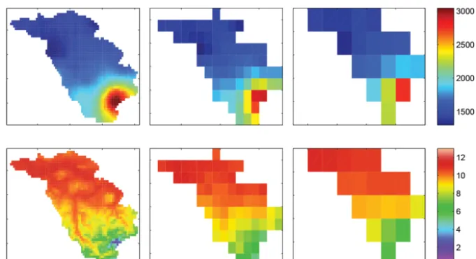
Figure 3.Upper panels: the precipitation sum in the Thur catchment over the full model period (1 August 2002–31 August 2003) shown for

different resolutions (f.l.t.r.: 1 km×1 km, 5 km×5 km, 10 km×10 km). Lower panels: the average temperature over this period for the same

spatial resolutions.

been obtained using a stage–discharge relation, based on several measurements conducted by FOEN throughout the years, amongst others, with an ADCP. The discharge mea-surements for the Rietholzbach catchment were made avail-able by ETH Zürich.

2.3 Forcing data

Forcing data for this study were made available by the Swiss Federal Office for Meteorology and Climatology (Me-teoSwiss). These data have previously been used for numer-ous applications of hydrological models in the Thur (Jasper et al., 2004; Abbaspour et al., 2007; Fundel and Zappa, 2011; Fundel et al., 2013; Jörg-Hess et al., 2015). The data are available for this study in the form required to implement the PREVAH model (Viviroli et al., 2009a, b). Data from nine different meteorological stations throughout the catchment (Güttingen, Hörnli, Reckenholz, Säntis, St. Gallen, Tänikon, Wädenswil, Zürich and Rietholzbach) were available with an hourly time resolution and spatially interpolated with the use of the WINMET tool of the PREVAH modelling sys-tem (Viviroli et al., 2009a), using elevation-dependent re-gression (EDR) and inverse distance weighting (IDW) and combinations of IDW and EDR. The data are available for the period 1981–2004, for which a stable configuration of stations is available. In this study, we only used data for the period May 2002–August 2003. To force the VIC model, hourly precipitation, incoming shortwave radiation, temper-ature, vapour pressure and wind data were used. We have run the model with two set-ups: fed with uniform forcing and fed with distributed forcing. Because the Thur basin has an extent of approximately 0.5◦, a lumped application of the forcing mimics the use of global forcing data sets like the WATCH forcing product and the ERA-Interim product.

Ap-plication with distributed forcing implied different forcing inputs for each grid cell. Because of the pronounced eleva-tion differences in the basin, precipitaeleva-tion and temperature show a clear spatial pattern, which can be seen in Fig. 3. 2.4 Spatial data for the model

Land use, hydraulic conductivity, elevation, and soil wa-ter storage capacity maps, all with a spatial resolution of 200 m×200 m, were provided by the Swiss Federal Institute for Forest, Snow and Landscape Research (WSL) under li-cense by swisstopo (JA100118). Also in this case we used the pre-processing routines created to implement the PREVAH modelling system (Viviroli et al., 2009a). The resolution of the available data (200 m×200 m) is higher than the model with the highest resolution in this study (1 km×1 km), which allows for sub-grid variability in the VIC model for land use and elevation parameters (see Sect. 3.1). Other soil charac-teristics, such as bulk density, have been obtained from the Harmonized World Soil Database (FAO et al., 2012), which has a spatial resolution of 1 km×1 km.

3 Model and routing description

3.1 The VIC model

The VIC model (Liang et al., 1994, 1996) is a land-surface model that solves the water and the energy balance. Subgrid land-use type variability is accounted for by providing veg-etation tiles that each cover a certain percentage of the total surface area. Three different types of evaporation are consid-ered by the VIC model: evaporation from the bare soil (Eb),

transpiration by the vegetation (T), considered per vegetation tile, and evaporation from interception (Ei). The total

evap-otranspiration is the area-weighted sum of the three evapo-ration types. The fraction of land that is not assigned to a particular land-use type is considered to be bare soil. Evap-oration from bare soil only occurs at the top layer (layer 1). If layer 1 is saturated, bare soil evaporation is at its poten-tial rate. Potenpoten-tial evaporation is obtained with the Penman– Monteith equation. If the top layer is not saturated, an Arno formulation (Francini and Pacciani, 1991), which uses the structure of the Xinanjiang model (Zhao et al., 1980), is used to reduce the evaporation.

For the upper two soil layers, the Xinanjiang formulation (Zhao et al., 1980) is used to describe infiltration. This for-mulation assumes that the infiltration capacity varies within an area. Surface runoff occurs when precipitation added to the soil moisture of layers 1 and 2 exceeds the local infiltra-tion capacity of the soil. Moisture transport from layer 1 to layer 2 and from layer 2 to layer 3 is gravity driven and only dictated by the moisture level of the upper layer. It is assumed that there is no diffusion between the different layers. Layer 3 characterizes long-term soil moisture response, e.g. season-ality. It only responds to short-term rainfall when both top layers are fully saturated. The gravity-driven moisture move-ment is regulated by the Brooks–Corey relationship:

Qi,i+1=Ksat,i

_W

i−Wr,i

W_ic−Wr,i

expti

. (1)

Qi,i+1 is the flow [L3T−1] from layer i to layer i+1. Ksat,iis the saturated hydraulic conductivity of layeri,Wi is

the soil moisture content in layeri,W_icis the maximum soil moisture content in layer i, andWr,i the residual moisture

content in layer i. The exponent of the Brooks–Corey rela-tion, expti, is defined as follows: _B2_p+3, in whichBpis the

pore size distribution index. The exponent as a whole is often calibrated.

Baseflow is determined based on the moisture level of layer 3. Baseflow generation follows the conceptualization of the Arno model (Francini and Pacciani, 1991). This for-mulation consists of a linear part (lower moisture content re-gions) and a quadratic part (in the higher moisture rere-gions). Baseflow is modelled as follows:

Qb=

   

  

dsdm

wsW3c

·W3 if 0≤W3≤wsW3c

dsdm

wsW3c

·W3+

dm−

dsdm

ws

W3−wsW3c

Wc

3−wsW3c

g

ifW3≥wsW3c

.

In this equation,Qbis the total baseflow over the model time step (in this study, 1 h),dmis the maximum baseflow,dsis the fraction ofdmwhere non-linear baseflow begins, andws is the fraction of soil moisture where non-linear baseflow starts.

W₃c is the maximum soil moisture content in layer 3, calcu-lated as a product of porosity and depth. The exponentgis by default set to 2 (Liang et al., 1996).

Since the grid size of the VIC model is often larger than the characteristic scale of snow processes, sub-grid variability is accounted for by means of elevation bands. For each grid cell the percentage of area within certain altitude ranges is pro-vided. The snow model is applied for each elevation band and land-use type separately; the weighted average provides the output per grid cell. This output consists of the snow wa-ter equivalent (SWE) and the snow depth. The snow model is a two-layer accumulation–ablation model, which solves both the energy and the mass balance. At the top layer of the snow cover the energy exchange takes place. A zero energy flux boundary is assumed at the snow–ground interface. A com-plete description of the model can be found in Liang et al. (1994, 1996).

3.2 Routing

The mizuRoute routine (Mizukami et al., 2015) takes care of the transport of water between the different grid cells. The routing is based on the same concept as the routing described by Lohmann et al. (1996), except that in mizuRoute the re-sponse is determined per subcatchment instead of per grid cell.

With the linearized St. Venant equation,

∂Q

∂t =D

∂2Q ∂x2 −C

∂Q

∂x, (2)

water is transported from the boundary of the subcatchment to the next subcatchment and finally to the outlet. In Eq. (2),

D(m2s−1) represents the diffusion coefficient andC(m s−1) the advection coefficient.

In the Thur basin, the routing is applied to subcatchments of the order of 1 km2. It is important to note that with the applied routing set-up, the drainage network is kept inde-pendent of the resolution, because surface runoff is routed for pre-defined sub-basins instead of per grid cell. In the de-fault VIC routing of Lohmann et al. (1996), water is routed per grid cell and is therefore dependent on the spatial reso-lution of the VIC model. By applying mizuRoute based on pre-defined sub-basins (∼1 km2), we have excluded the ef-fect of the spatial resolution on the routing process.

4 Experimental set-up

M J J A S O N D J F M A M J J A S 0

100 200 300 400 500 600

Discharge (m

3s

−1

)

Model period Spin−up period Model runs

0 20 40 60 80 100

0 100 200 300 400 500 600

Exceedance (%)

Discharge (m

3s

−1

)

Flow duration curve 39 yr. Covered in model period

Figure 4.Daily discharge characteristics for the Thur basin. Left panel: the daily discharge in the Thur for the selected model period. The

black lines show three model runs with the same parameter set but with different initial conditions (θ=0.5, 0.7, 0.9). Right panel: part of

the flow duration curve covered within the model period. The flow duration curve is based on 39 years of daily discharge observations in the Thur basin for the period 1974–2012.

both uniform and distributed forcing. Since for the lumped model there is no difference between uniform and distributed forcing, this leads to a total of seven different model set-ups. Because the runtime of the model combined with all the post-processing is rather long (on average 2.5 h for the 1 km×1 km model on a standard PC), an efficient sampling strategy was designed. The procedure we followed is illus-trated in Fig. 5. With sensitivity analysis (Sect. 4.4) the most sensitive parameters from the model were selected. Subse-quently, we sampled the full parameter space with a uni-form prior using the Hierarchical Latin Hypercube Sam-ple (HLHS) (Vorˆechovský, 2015); see Sect. 4.5. Although sampling the parameter space with a uniform prior is less efficient than other distributions which focus more on the most likely regions, we did not want to exclude any region because both the temporal and spatial resolution were var-ied. The sampled parameters were applied uniformly over the catchment, whereas all other soil- and land-use parame-ters have been applied in a distributed fashion. After running the models with the HLHS, the output was evaluated and the best 1 % of the runs was defined as behavioural. The over-lap in behavioural sets was used as an indicator of parameter transferability (Sect. 4.7).

4.1 Spatial model resolution

Four VIC implementations with different spatial reso-lutions (0.0109◦ roughly corresponding to 1 km×1 km, 0.0558◦≈5 km×5 km, 0.1100◦≈10 km×10 km, as well as a lumped model) were constructed. The 1 km×1 km model represents the so-called hyper-resolution. Several studies already explore GHMs at this resolution, e.g. Su-tanudjaja et al. (2014) for the Rhine–Meuse basin. The model with the 10 km×10 km resolution can be characterized as “regional”. The 5 km×5 km model is in between the hyper-resolution scale and the regional scale. The lumped model, which represents an area of 1703 km2, is of the order of mag-nitude of grid cells with a 0.5◦resolution, which represents the original scale for which VIC was developed. Figure 1 gives an overview of the cell size of the four models. The

sampled parameters (see Sect. 4.4) have been applied uni-formly over the catchment; all other parameters have been applied in a distributed manner. We will discuss the effect of applying the sampled parameters uniformly by using data from the nine subcatchments.

4.2 Temporal model resolution

The models are run at an hourly time step, implying that they solve both the energy and the water balance. The hourly out-put of the routing model is aggregated to daily and monthly time steps for further evaluation; see Fig. 1.

4.3 Simulation period

The four models are run for a period of 1 year and 4 months. The first 3 months are used as a spin-up period and are not used for further analysis. Tests with the same parameter set and different initial conditions revealed that 3 months are suf-ficient to eliminate the effect of initial conditions (see Fig. 4). The initial soil moisture content of the model before spin-up was fixed atθ=0.9 because we found that the model reaches equilibrium faster when starting from a wet state. The models have not been subjected to a validation procedure on another time period, because in this particular application the goal was not to identify the best performing model, but to investi-gate the role of temporal and spatial resolution in parameter transferability.

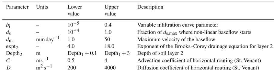
Senevi-Table 1.Sampled model parameters.

Parameter Units Lower Upper Description

value value

bi – 10−5 0.4 Variable infiltration curve parameter

ds – 10−4 1.0 Fraction ofds,maxwhere non-linear baseflow starts

dm mm day−1 1.0 50 Maximum velocity of the baseflow

expt2 – 4.0 18.0 Exponent of the Brooks–Corey drainage equation for layer 2

Depth2 m Depth1+0.1 Depth1+3 Depth of soil layer 2

C ms−1 0.5 4 Advection coefficient of horizontal routing (St. Venant)

D m2s−1 200 4000 Diffusion coefficient of horizontal routing (St. Venant)

ratne et al., 2012). With these two extremes the selected pe-riod covers a large part of the flow duration curve, in both the high and low flow regions (right panel in Fig. 4).

4.4 Model parameters

The VIC model has a large number of parameters, divided over three sections: soil parameters, vegetation parameters, and snow parameters. To determine which parameters should be sampled in this study, a sensitivity analysis was conducted on a broad selection of parameters (see Table S1 in the Sup-plement). The parameter selection was made such that the main hydrological processes were represented and included 28 VIC parameters from the three different sections. Sensi-tivity analysis was conducted using the distributed evalua-tion of local sensitivity analysis (DELSA) method (Rakovec et al., 2014). DELSA is a hybrid local–global sensitivity analysis method. It evaluates parameter sensitivity based on the gradients of the objective function for each individual parameter at several points throughout the parameter space. Note that this method only provides first-order sensitivities and thus does not account for parameter interaction.

A base set of 100 parameter samples was created. For each parameterkthat is accounted for in the analysis, the base set of parameter samples is perturbed. In total, including the base set, this leads to (number of parameters+1)×100 parameter samples that need to be evaluated. To save computation time, the sensitivity analysis was conducted on the lumped VIC model for the Thur basin. To study the effect of spatial scale on sensitivity, two lumped models for subbasins of the Thur have been constructed: the Jonschwil catchment (495 km2) and the Rietholzbach catchment (3.3 km2). The Rietholzbach catchment is nested inside the Jonschwil catchment, which is again nested in the Thur catchment (Fig. 2). The three catchments have comparable land use. The Kling–Gupta effi-ciency of the discharge (KGE(Q)), Nash–Sutcliffe efficiency of the discharge (NSE(Q)) and the Nash–Sutcliffe efficiency of the logarithm of the discharge (NSE(logQ)) (see Sect. 4.6) were used as objective functions to assess the sensitivity of the parameters.

The analysis showed that parameter sensitivity did not no-tably change over the assessed scales: the same parameters

were found to be most sensitive, but in a slightly differ-ent order (see Fig. S1 in the Supplemdiffer-ent). There are four parameters which, for all scales and for all objective func-tions, proved to be highly sensitive: the parameter describ-ing variable infiltration (bi), the parameter that defines the fraction ofds,max where non-linear baseflow starts (ds), the

maximum velocity of the baseflow (dm) and the exponent of

the Brooks–Corey relation (_B2

p +3, expt2; see Eq. 1). Hence,

these four parameters were selected for the sampling analy-sis. Other parameters that showed sensitivity in some cases were the depth and bulk density of soil layer 2, the depth and bulk density of soil layer 3, and the rooting depth of layer 1. The selection of sensitive parameters closely resembles the results of Demaria et al. (2007), who applied a sensitivity analysis to VIC over different hydroclimatological regimes. Because Demaria et al. (2007) found that the depth of soil layer 2 was highly sensitive, this parameter was added to the selection of parameters that was sampled. In addition, the two routing parametersCandDwere sampled because they control the lateral exchange of water between grid cells. An overview of the selected parameters is given in Table 1. Be-cause sampling the seven selected parameters in a distributed fashion is computationally extremely demanding and cur-rently not yet feasible, the sampled parameters have been ap-plied uniformly over the cells in the distributed VIC models. This is according to current practice in large-scale modelling.

4.5 Hierarchical Latin Hypercube Sample

P1

P2 P3

P1 P2 P3 P1 P2 P3 P1 P2 P3

P3

P2

P1 P2 P3

P3

P2

(a) (b) (c) (d)

Figure 5.Parameter sampling as applied in this study.(a)Example situation when sampling for a model with three parameters.(b)

Sen-sitivity analysis can be conducted to decrease the dimensions of the sampling space.(c)Latin Hypercube sampling is structured and more

efficient: one sample in each row and each column, as indicated with the bands. The number of samples has to be determined beforehand.

(d)Hierarchical Latin Hypercube Sampling allows to extend the sample if necessary, while conserving Latin hypercube structure.

while still being able to provide insights into e.g. posterior parameter distributions. For a Monte Carlo (MC) sample, it is easy to start with a small sample, and add more samples if this proves to be necessary, e.g. based on the sample variance. For a variance reduction technique such as LHS this is not that straightforward. Therefore, we make use of the Hierar-chical Latin Hypercube Sample (HLHS), recently developed by Vorˆechovský (2015). This method allows us to start with a small LHS and add more samples if necessary, while con-serving the LHS structure (Fig. 5d). Inherent to this method is that every sample extension is twice as large as the previ-ous sample, which results in a total number of simulations afterrextensions:

Nsim,r=3r·Nstart, (3)

withNsim being the total number of simulations,rthe

num-ber of extensions, andNstartthe start number of samples. As a

starting sample size, 350 is chosen, which is sampled based on a space-filling criterion. For the seven parameters in the HLHS a uniform prior is assumed in order the study the full parameter space. The starting sample can be increased by a first extension to 1050 samples in total, further to 3150, and even up to 9450. After each extension, the cumulative dis-tribution function (CDF) of the objective functions (KGE, NSE) is compared with the CDF of the previous extension. A Kolmogorov–Smirnov test is used to test whether the CDFs are significantly different. It was found that the CDF es-timated from 3150 samples was not significantly different from the CDF based on 1050 samples at a 0.05 significance level. Therefore, 3150 samples were considered sufficient to sample the parameter space.

4.6 Objective functions

For each model run, several objective functions were evalu-ated. The three objective functions are

– the Kling–Gupta efficiency (KGE) to describe the over-all capability of the model to simulate the discharge

(Gupta et al., 2009): KGE(Q)=1−

q

(r−1)2_+(α−1)2_+(β−1)2_{, (4)}

where r is the correlation between observed dis-chargeQoand modelled discharge Qm,α is the stan-dard deviation ofQmdivided by the standard deviation ofQo, andβ is the mean ofQm(Qm) divided by the

mean ofQo(Qo);

– the Nash–Sutcliffe efficiency (NSE) of the discharge to describe the model performance for the higher dis-charge regions (Nash and Sutcliffe, 1970):

NSE(Q)=1−

T P

t=1

Qt_o−Qt_m2

T P

t=1

Qt_o−Q_o2

=2·α·r−α2−β_n2, (5)

in whichβnis the bias normalized by the standard devi-ation; and

– the Nash–Sutcliffe efficiency of the logarithm of the dis-charge NSE(logQ) to test the model performance for low discharges (Krause et al., 2005).

The objective functions are calculated for all runs (3150) for the seven different VIC set-ups and based on hourly, daily and monthly time steps.

4.7 Determination of behavioural sets and parameter transferability

1x1 km 5x5 km 10x10 km L 0.3

0.4 0.5 0.6 0.7 0.8 0.9

Resolution

KGE(Q)

Hour (uniform | distributed forcing) Day (uniform | distributed forcing) Month (uniform | distributed forcing)

1x1 km 5x5 km 10x10 km L

0.3 0.4 0.5 0.6 0.7 0.8 0.9

Resolution

NSE(Q)

1x1 km 5x5 km 10x10 km L

0.3 0.4 0.5 0.6 0.7 0.8 0.9

Resolution

NSE(logQ)

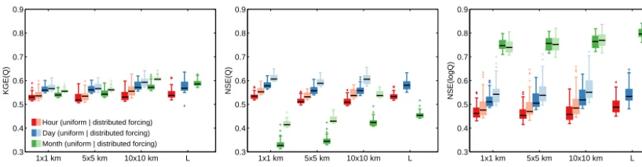
Figure 6. Model performance of the behavioural sets for different temporal resolutions and different spatial resolutions. The left panel

shows the KGE(Q), the middle panel the NSE(Q) and the right panel the NSE(logQ). Per objective function the most behavioural sets were

selected; hence, the selected sets where not necessarily the same for the three objective functions. The box shows the 25th–75th percentiles. .

the three objective functions separately, the 32 best mem-bers are selected. We evaluate all 32 parameter sets as be-ing equally plausible and do not assign weights to the best performing sets within the behavioural selection, to account for uncertainty in the observations. Inherent to our approach, selecting a certain percentage of runs rather than applying a threshold level based on an objective function, is that the selected runs do not necessarily comply with an acceptable model performance. We expect that this neither positively nor negatively influences our results concerning parameter transferability.

We define parameter transferability θ↔ as the percentage

agreement in selected behavioural sets:

θ

↔=# ASi,Tj∩BSk,Tl

/n·100, (6)

in which ASi,Tj is the set of selected behavioural members for spatial resolution Si and temporal resolution Tj, and BSk,Tl are the selected members for spatial resolutionSkand temporal resolutionTl. Thenis the total number of selected

members (in this case, 32). Equation (6) expressesθ_↔as a per-centage; ifθ_↔=100, this indicates that for two different res-olutions (either spatial, temporal or both), exactly the same parameter sets were selected as behavioural.

5 Results

First, the impact of temporal and spatial resolution on model performance is discussed for both uniform and distributed forcing, followed by a discussion of the impact of the tempo-ral and spatial resolution on parameter distribution. For these analyses, the temporal and spatial resolution are assumed to be independent. Subsequently, the parameter transferability across temporal and spatial resolution is assessed by deter-mining the overlap in behavioural sets as defined by Eq. (6). After that, parameter transferability over both temporal and spatial resolution is assessed. Finally, we investigate param-eter transferability over the sub-basins of the Thur.

5.1 Impact of temporal and spatial resolution on model performance and parameter distribution

Figure 6 shows the model performance of the behavioural sets for the different spatial and temporal resolutions and the different objective functions, both for uniform and dis-tributed forcing. We will first discuss the results for the uni-form forcing.

With uniform forcing, the lumped model outperforms the distributed models for all three objective functions and time steps. The monthly time step shows for all three objective functions an increasing model performance with decreasing spatial resolution. It is remarkable that the model with the monthly time step outperforms the models with daily and hourly time steps when the NSE(logQ) was used as an ob-jective function, while with the NSE(Q) as an objective func-tion exactly the opposite is the case. It is important to notice here that the monthly model results are simply an aggrega-tion from the hourly model results, which might imply that the higher score on the monthly time step is the result of er-rors which compensate for each other, and that the model performance scores for the monthly time step are based on a considerable lower number of points. The KGE(Q) as an objective function does not lead to a significantly different model performance for the monthly time step. From the fig-ure it seems that both the spatial and temporal resolution have impact on the model performance. This is confirmed with a statistical test. An ANOVA analysis with two factors (temporal resolution, spatial resolution), with three or four levels (hourly, daily, monthly; 1 km×1 km, 5 km×5 km, 10 km×10 km and lumped) shows that both the spatial and temporal resolution have a significant (p <0.05) impact on all three objective functions.

1x1 km 5x5 km 10x10 km L 0.7

0.75 0.8 0.85 0.9 0.95 1

Resolution

Correlation (r)

1x1 km 5x5 km 10x10 km L

0 0.5 1 1.5 2

Resolution

St

d

e

v

(m

o

d

)/

s

td

e

v

(o

b

s

) (

α

)

Hour (uniform | distributed forcing) Day (uniform | distributed forcing) Month (uniform | distributed forcing)

1x1 km 5x5 km 10x10 km L

1 1.2 1.4 1.6 1.8 2

Resolution

M

e

a

n

(m

o

d

)/

m

e

a

n

(o

b

s

) (

β

)

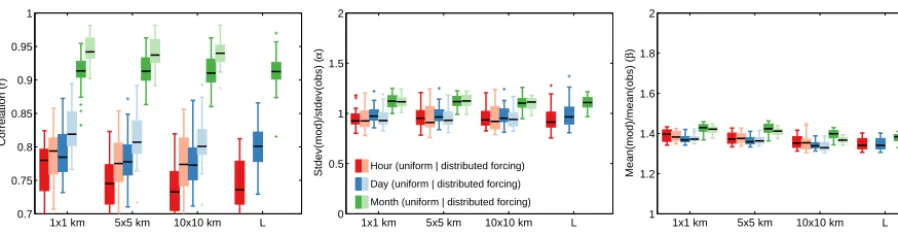
Figure 7.The model performance for the three separate components of the Kling–Gupta efficiency of the behavioural sets for different

temporal and spatial resolutions. The left panel shows the correlationr, the middle panel the standard deviation of the model output divided

by the standard deviation of the observations (α), and the right panel shows the mean of the model output divided by the mean of the

observations (β).

the other model set-ups, for the distributed forcing the 10 km×10 km model outperforms the other spatial resolu-tions (except for NSE(logQ)). An ANOVA analysis con-firmed that also for distributed forcing, both spatial and tem-poral resolution have a significant (p <0.05) impact on the model performance for all three objective functions.

Figure 7 shows the distribution of the behavioural sets for the three separate components of the KGE(Q). Regarding the correlation r, the monthly time step scores higher than the daily and hourly time step. On the other hand, the hourly and daily time steps score higher with respect toβ (closer towards 1). Although Fig. 6 gives the impression that the model performance in terms of KGE(Q) is relatively insen-sitive to temporal and spatial resolution, Fig. 7 reveals this is actually the result of compensations from the three differ-ent compondiffer-ents of the KGE(Q): the monthly time step has a higher correlation, while the daily and hourly time steps have a higherβ.

Figure 8 shows the parameter distribution of the seven sampled parameters, and shows how the distribution varies as a function of temporal and spatial resolution, both for distributed and uniform forcing. The distribution of the be-havioural parameter sets for the daily and hourly time steps are very much alike for all parameters, but the distribution for the monthly time step is in some cases broader, which implies that the parameters are less clearly defined. The pa-rameter showing the clearest effect of temporal scale is the advection coefficientC(Fig. 8). TheCparameter, the veloc-ity component in the routing, becomes less well defined with an increasing time step, which is intuitive because timing be-comes less relevant for longer time intervals.

The difference in the parameter distribution when com-paring distributed and uniform forcing is limited. The clear-est difference can be found for the dm parameter with the NSE(Q) as an objective function. This parameter describes the maximum velocity of the baseflow, and can potentially impact short-term processes for which distributed forcing seems important, like surface runoff. However, there are

other parameters, such as thebi parameter, which are more directly linked to infiltration and surface runoff processes and do not show a clear difference in parameter distribution be-tween distributed and uniform forcing.

With an ANOVA analysis, the significance of temporal and spatial resolutions in the parameter distribution of the behavioural sets was tested. Figure 9 shows that the signif-icance of spatial and temporal resolutions in the parameter distribution depends on which objective function was used to determine the behavioural sets. Uniform and distributed forcings show comparable patterns. In general, the temporal resolution has more impact on the parameter distribution (at least four parameters are significantly affected by temporal resolution) than the spatial resolution (only one parameter for one objective function experiences significant impact of the spatial resolution). Only two parameters are significantly impacted by the temporal resolution for all three objective functions:dsandC.

5.2 Parameter transferability

The main research question of this study is to what extent parameters are transferable across temporal and spatial reso-lutions, and we will use that as an indicator of the representa-tion of spatial and temporal variability in the model. We have defined parameter transferabilityθ↔as the percentage

agree-ment in identified behavioural sets (Eq. 6). Tables 2 and 3 give an overview ofθ↔for different temporal and spatial

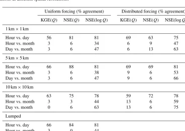
res-olutions, both for uniform and distributed forcing. Table 2 shows that theθ↔ is generally high for different spatial

0.1 0.2 0.3 0.4 0

5 Original sampledistribution

↓

0.1 0.2 0.3 0.4

0 10 20

0.1 0.2 0.3 0.4

0 2 4

0.2 0.4 0.6 0.8 1

0 10 20 30

0.2 0.4 0.6 0.8 1

0 10 20 30

0.2 0.4 0.6 0.8 1

0 10 20 30

10 20 30 40 50

0 0.5

Hour (unif. | distr. forcing) Day (unif. | distr. forcing) Month (unif. | distr. forcing)

10 20 30 40 50

0 0.05 0.1

10 20 30 40 50

0 0.02 0.04

5 10 15

0 0.2 0.4

5 10 15

0 0.2 0.4

5 10 15

0 0.1 0.2

0.5 1 1.5 2 2.5 3

0 1 2

0.5 1 1.5 2 2.5 3

0 1 2

0.5 1 1.5 2 2.5 3

0 1 2

1 2 3 4

0 0.5 1

1 2 3 4

0 2 4

1 2 3 4

0 0.5 1

1000 2000 3000 4000

0 2 4x 10

−4

1000 2000 3000 4000

0 5x 10

−4

1000 2000 3000 4000

0 5x 10

−4

Density

Density

Density

Density

Density

Density

Density

b_i (−)

d

s (−)

d

m (mm d

−1₎

expt

2 (−)

Depth₂ (m)

C (ms−1)

D (m2s−1)

KGE(Q) NSE(Q) NSE(logQ)

Figure 8.Distribution of the sampled parameters for the behavioural sets, fitted with a kernel density. The width of the line indicates the

variation in distribution between the different spatial resolutions. The left column is based on KGE(Q), the middle column on NSE(Q) and

the right column on NSE(logQ).

is that the NSE(logQ) tends to put more focus on lower dis-charges with a longer timescale, with less focus on the short-term flashy response of a catchment. Parameter transferabil-ity over space is in general slightly lower when distributed forcing is used compared to uniform forcing. On the other hand, parameter transferability over time is slightly higher for distributed forcing. Decreased sensitivity for the temporal resolution and increased sensitivity for the spatial resolution can indicate an improved physical representation with

dis-tributed forcing compared to uniform forcing, as one would expect.

Table 2.Transferability of parameters across spatial resolution, expressed as percentage agreement in detected behavioural runs for different spatial resolutions (in km) at different time steps.

Uniform forcing (% agreement) Distributed forcing (% agreement)

KGE(Q) NSE(Q) NSE(logQ) KGE(Q) NSE(Q) NSE(logQ)

Hour

1×1 vs. 5×5 78 84 91 88 75 84

1×1 vs. 10×10 72 81 81 78 56 78

5×5 vs. 10×10 94 94 91 88 81 94

1×1 vs. lumped 78 88 91

5×5 vs. lumped 91 84 94

10×10 vs. lumped 88 81 88

Day

1×1 vs. 5×5 94 84 84 91 84 91

1×1 vs. 10×10 84 69 69 78 69 81

5×5 vs. 10×10 91 84 84 89 84 91

1×1 vs. lumped 1 81 88

5×5 vs. lumped 91 88 94

10×10 vs. lumped 84 84 81

Month

1×1 vs. 5×5 75 88 88 84 84 91

1×1 vs. 10×10 66 84 81 66 78 84

5×5 vs. 10×10 88 91 94 78 88 94

1×1 vs. lumped 78 72 94

5×5 vs. lumped 78 75 88

10×10 vs. lumped 78 78 88

Table 3.Transferability of parameters across temporal resolution, expressed as percentage agreement in detected behavioural runs for

differ-ent temporal resolutions at differdiffer-ent spatial resolutions.

Uniform forcing (% agreement) Distributed forcing (% agreement)

KGE(Q) NSE(Q) NSE(logQ) KGE(Q) NSE(Q) NSE(logQ)

1 km×1 km

Hour vs. day 56 81 81 69 63 75

Hour vs. month 3 6 34 6 9 47

Day vs. month 3 6 47 6 13 63

5 km×5 km

Hour vs. day 66 88 81 69 69 81

Hour vs. month 3 6 38 9 6 53

Day vs. month 3 6 47 9 6 66

10 km×10 km

Hour vs. day 63 75 78 59 72 78

Hour vs. month 3 3 44 13 6 59

Day vs. month 0 6 63 13 6 75

Lumped

Hour vs. day 66 84 81

Hour vs. month 3 0 44

p−value 0.02 0.04 0.06 0.08 0.1 0.12 KGE(Q) NSE(Q) NSE(logQ)

S T S T S T

b_i d s d_m expt₂ Depth₂ C D Uniform forcing p−value 0.02 0.04 0.06 0.08 0.1 0.12 KGE(Q) NSE(Q) NSE(logQ)

S T S T S T

Distributed forcing

Figure 9.The effect of spatial and temporal resolutions on

parame-ter distribution. Thepvalue indicates the significance of the impact

of spatial resolution (S) and temporal resolution (T) on the

param-eter values of the behavioural sets, evaluated for the three objective functions.

through the data points from our study (R2=0.68). The fig-ure clearly shows that temporal resolution has a stronger impact on parameter transferability than spatial resolution. The linear regression equation that describes the surface in Fig. 10 is given below:

θ

↔KGE(Q)=83.3−12.6·

Tj Tl

−3.0·Si

Sk

, (7)

in which Tj

Tl is the ratio in temporal resolution between the two model set-ups over which parameters are trans-ferred and Si

Sk is the ratio in spatial resolution (L/L) be-tween the two model set-ups. The effect of temporal reso-lution on parameter transferability is stronger (slope of 12.6) than the effect of spatial resolution (slope of 3.0). Parameter transferability decreases when the ratio between the original and the intended spatial and temporal resolutions increases. The surfaces based on NSE(Q) (R2=0.60) and NSE(logQ) (R2=0.75) show a similar behaviour:

θ

↔NSE(Q)=88.6−12.8·

Tj Tl

−2.8·Si

Sk

, (8)

θ

↔_NSE(logQ)=92.9−7.4· Tj

Tl

−3.6·Si

Sk

. (9)

When we fit a surface through the points obtained for the models run with distributed forcing, the linear regression equations (R2=0.66, 0.67, 0.88 respectively) look as fol-lows:

θ

↔_KGE(Q)=80.3−11.4· Tj Tl

−2.6·Si

Sk

, (10)

θ

↔NSE(Q)=75.3−10.3·

Tj Tl

−4.3·Si

Sk

, (11)

θ

↔NSE(logQ)=91.3−5.4·

Tj

Tl

−2.8·Si

Sk

. (12)

Also for the models with distributed forcing, the slope for the temporal resolution is steeper than the slope for spatial reso-lution, implying that parameter transferability is more sensi-tive for temporal resolution than for spatial resolution. Com-pared to uniform forcing, the slope for temporal resolution,

O

ver

lap in beha

viour

al par

amet

er sets (%)

100 90 80 70 60 50 40 30 20 10 0 Increasing r atio spa tial resolution Increasing r atio tempor

al resolution

Figure 10.Parameter transferability as a function of the ratio in

temporal and spatial resolution. The ratio of temporal resolutions is defined as follows: transfer from hourly to daily time steps is a ratio of 24, whereas transfer from hourly to monthly is a ratio of 732 (732 h in 1 month of 30.5 days). The ratio of spatial resolutions is defined as the square root of the number of cells that would fit in the

other cell: from 1 km×1 km resolution to 5 km×5 km resolution is

a ratio of

√

25=5. The behavioural sets were determined based on

the KGE(Q). The linear surface (R2=0.68) was fitted to illustrate

the relative impact of changes in spatial and temporal resolution.

and hence the impact of temporal resolution on transferabil-ity, is less steep for distributed forcing, while the slope for spatial resolution is on average comparable for both forcings. 5.3 Spatially distributed parameters

vari-Table 4.Transferability of parameters from the Thur to the nine subbasins, expressed as percentage agreement (%) in detected behavioural

runs. The forcing was applied uniformly and the KGE(Q) was used as an objective function.

Catchment (size) 1 km×1 km 5 km×5 km 10 km×10 km

Hour Day Month Hour Hour

Rietholzbach (3.3 km2) 19 0 0 25 19

Herisau (17.8 km2) 16 6 0 16 16

Appenzell (74.2 km2) 28 25 9 28 16

Wängi (78.9 km2) 9 56 31 34 50

Mogelsberg (88.2 km2) 28 38 66 19 28

Frauenfeld (212 km2) 3 3 75 3 0

St. Gallen (261 km2) 3 0 0 3 0

Jonschwil (493 km2) 6 0 0 6 0

Halden (1085 km2) 19 9 0 18 13

ation in the calibrated parameters is underestimated in the current model set-up.

6 Discussion

6.1 Model performance

It seems counter-intuitive that model performance is signif-icantly affected by both the temporal and spatial resolution, while the parameter distribution is mainly impacted by the temporal resolution. This can be explained, however. Model performance can still be significantly impacted by temporal and spatial resolution, even if the same parameters are se-lected for different spatial resolutions. This implies that the model performance is mainly limited by the model structure or set-up, and much less by the parameter values. This is confirmed by comparing the uniform and distributed forc-ing. Although the distribution of the behavioural parameters was not very different for the two forcing types, the model performance for distributed forcing was in almost all cases better than the model performance for the uniform forcing.

Liang et al. (2004) defined a so-called “critical resolution”, beyond which a finer spatial resolution would not lead to any improvement in the model performance. In the study of Liang et al. (2004) this critical resolution for the VIC model was found to be 1/8◦(≈12.5 km×12.5 km). All spa-tial resolutions applied in this study, but the lumped ones are below this critical resolution. The results in this study are therefore consistent with the results from Liang et al. (2004), because we did not find any improvement in model per-formance with increasing spatial resolution, neither for the uniform nor for the distributed forcing. Rather, we find the contrary; for the uniform forcing the lumped model outper-formed the higher-resolution models, and for the distributed forcing the 10 km×10 km outperformed the other models. If something like a critical resolution exists, it is proba-bly related to the processes represented in the model.

Con-trary to our findings are the results of Zappa (2002), who found that a critical spatial resolution in the Thur region is of the order of 500 m×500 m using the PREVAH model, be-cause of the complex topography and snow processes in the catchment. This can either imply that the sub-grid variability parametrization in VIC is effective, or that not all relevant hy-drological processes are included in the VIC model. In order to check this last suggestion, future research on parameter transferability should consider more hydrological fluxes and states besides the discharge, e.g. evapotranspiration. 6.2 The high sensitivity for temporal resolution

1x1 km 5x5 km 10x10 km L 1350

1400 1450 1500 1550 1600 1650 1700 1750

Resolution

Bulk density layer 1 (kg m

−3

)

Figure 11.Distribution of bulk density over the grid cells for the

four different spatial resolutions.

the temporal resolution. They found that the sensitivity of a parameter to temporal resolution could be related to the model structure; the parameters from simpler model struc-tures were more sensitive to temporal resolution than the pa-rameters from more complex models.

Figure 12 and Tables S2 and S3 show that the conclusions we draw from Tables 2 and 3 are not only valid for the best 1 % of runs selected as behavioural. Tables S2 and S3 show that the same patterns are found when selecting the best 2 % or 5 % of the model runs. Figure 12 gives an overview for two selected cases, which show that model performance de-teriorates when parameters are transferred over time, also for the best 10 % up to higher thresholds, whereas the impact of spatial resolution on model performance deterioration is limited.

6.3 Models vs. nature: do the current generation of models adequately represent spatial variability? Our results show that parameter transferability is more sen-sitive to temporal than to spatial resolution. A key question is to what extent this result stems from the model representa-tion of spatial variability. Spatial variability can be reflected in three domains of the model: the routing, the forcing, and the soil and land-use parameters. In this study we excluded the effect of routing by using a high-resolution drainage net-work based on sub-basins with a size of∼1 km2, indepen-dent of the resolution of the hydrologic model. We think that the effect of spatial resolution can be increased by adapt-ing the routadapt-ing scheme accordadapt-ingly. Drainage network res-olution may affect the projected hydrograph, for example with changes in the stream network and the channel slope. However, this effect should then be assigned to the routing model, and not to the runoff generation model (the hydro-logic model). For clarity, we decided to exclude the effect of spatial resolution on routing in this study.

We investigated the effect of forcing by comparing the re-sults for distributed and uniformly applied forcing, and we tested the effect of spatially distributed soil and land-use

pa-rameters by aggregating them for lower resolutions (Fig. 11). Despite distributed forcing and the decrease in variation in soil and land-use parameters, the model parameters showed low sensitivity to the spatial resolution. A possible explana-tion could be the sub-grid parametrizaexplana-tions of the VIC model for land use and elevation, which decrease the effect of up-scaling these parameters to other resolutions, as shown by Haddeland et al. (2002). However, we think that Sect. 5.3 and Table 4 show how spatial variability is underestimated by calibrating and applying the most sensitive parameters uni-formly over the basin.

The models in this study are configured in a similar way to many current-day large-domain hydrological models, us-ing common data like the Harmonized World Soil Database and uniform application of the most sensitive parameters. As such, this study is likely representative of many large-domain studies. The limited sensitivity for spatial resolution is arguable because our implementation of VIC substantially underestimates the spatial variability in nature, and, impor-tantly, that similar issues in representing spatial variability are a common problem in large-domain hydrological mod-elling (e.g. see the model configuration in Mizukami et al., 2016). Many studies have considered spatial variability in forcing (Adams et al., 2012; Lobligeois et al., 2014) and soil parameters (Mohanty and Skaggs, 2001; Western et al., 2004). Kim et al. (1997) accounted for heterogeneity in soil hydraulic properties using stochastic methods, based on the scaling theory of Miller and Miller (1956). In fact, the effect of stochastic soil parametrizations on parameter transferabil-ity would be a valuable research topic (Maxwell and Kollet, 2008). We argue here that the high spatial transferability may occur because the current generation of land-surface mod-els have an inadequate representation of spatial variability and hydrologic connectivity, providing a strong motivation to substantially improve the representation of spatial and tem-poral variability in models. This not only implies increasing the spatial (and temporal) resolution of the model, but also including more relevant hydrological processes. Promising techniques have been developed to allow spatial distribution of calibrated parameters, for example with multiscale param-eter regionalization (MPR, Samaniego et al., 2010; Kumar et al., 2013), which could and should be applied for large-domain hydrologic models.

6.4 Limitations of this case study

NSE(Q)

1KM

0 0.5

10KM

NSE(Q)

Relative frequency

10KM

0.0−0.1 quantile

0.9−1.0 quantile

0 0.5

Relative frequency

1KM

→

→

from to

SPACE

behavioural set (1%)

←

HOUR MONTH

Relative frequency

MONTH

Relative frequency

HOUR

→

→

from to

TIME

0.0 0.2 0.4 0.6 0.8 1.0

Original quantile of runs based on NSE(Q)

Figure 12.Impact of parameter transfer on model performance. The panels show the distribution of the NSE(Q) fitted with a kernel density

for 3150 runs. On the left-hand side of the arrow the red area represents the best 10 % of the runs, each colour interval increasing with 10 % to the full data set (100 %, purple). The selected behavioural runs are indicated separately with a black line (best 1 %). The panel on the right-hand side of the arrow shows the distribution of the model performance for the coloured selections when evaluated at another spatial (left panels) or temporal (right panels) resolution. When the direction of the colours changes from the left panel to the right panel, this implies a low parameter transferability. The data for the first two columns are based on hourly discharges; the data for the second two columns are

based on the 1 km×1 km model.

could be substantially underestimated. The impact of tempo-ral resolution on parameter transferability is large. We em-ployed the temporal resolutions for which most hydrological observations are available; thus, our results are relevant for practical applications. Based on the work of Chaney et al. (2015) we expect that parameter transferability will be lower for arid climates than the numbers we obtained, and based on the work of Kavetski et al. (2011) we expect that parameter transferability will be lower for more parsimonious models. The general message from our study is the surprisingly high spatial transferability, highlighting the need for a focused re-search effort to improve the representation of spatial vari-ability in large-domain distributed models (GHMs). A possi-ble path forward is to develop computationally frugal process representations, as for example presented by Hazenberg et al. (2015) for hillslope processes.

7 Summary and conclusions

A VIC model for the Thur basin was run with four different spatial resolutions (1 km×1 km, 5 km×5 km, 10 km×10 km, lumped) and evaluated at three different

tem-poral resolutions (hourly, daily, monthly). The forcing was applied both uniformly and distributed over the catchment, and the drainage network for the routing model was defined independently of the hydrological model resolution. Three objective functions were used to evaluate model perfor-mance: KGE(Q), NSE(Q) and the NSE(logQ). The model was run 3150 times using the Hierarchical Latin Hyper-cube Sample and the best 1 % of the runs was selected as behavioural and used for further analysis. Parameter trans-ferability was quantified by evaluating the overlap in be-havioural sets for different temporal and spatial resolutions. From the results we can draw the following conclusions.

– The spatial resolution of the model had little impact on the parameter distribution of the behavioural sets. On the other hand, the temporal resolution significantly impacted the distribution of at least four out of seven parameters, both when applied with uniform and dis-tributed forcing.

– Parameters could to a large extent be transferred across the spatial resolutions, while parameter transferability over the temporal resolutions was less trivial. Param-eter transferability between the hourly and daily time steps was found to be feasible, but the monthly time step led to substantially different parameter values. This is crucial information, because many studies tend to cali-brate the VIC model on the monthly time step (Melsen et al., 2016). The results of this study suggest that the output from models calibrated on a monthly time step cannot be interpreted or analysed on a daily or hourly time step. This might seem obvious, but it should be rec-ognized that the increasing spatial resolution of large-domain land-surface models might increase the expec-tations concerning temporal resolution as well, as de-scribed in Melsen et al. (2016).

– We also investigated whether parameters could be trans-ferred across both the spatial and the temporal res-olutions simultaneously. Parameter transferability de-creases when the ratio between the original and the in-tended spatial and/or temporal resolution increases. The ratio of temporal resolutions has a larger negative ef-fect on parameter transferability than the ratio of spa-tial resolutions. It was also shown that parameter trans-ferability depends on the objective function. When the NSE(logQ), which tends to put more emphasis on low flows, is used as an evaluation criterion, the parame-ter values at a monthly time step overlap much more with the daily and hourly time steps than when KGE(Q) or NSE(Q) are used as objective functions. This means that parameter transferability across temporal resolution also depends on the timescale of the process to which a particular parameter refers.

The most important result of our study is that it showed high parameter transferability across spatial resolution, even when forcing was applied in a distributed fashion. A possible ex-planation for the low sensitivity to spatial resolution is the uniform application of the most sensitive parameters. This is indicative of a substantial underestimation of the actual spatial variability represented by the VIC simulations. We did, however, construct our model according to current-day standards for large-domain land-surface models, raising the point that the high spatial transferability may occur because the current generation of models has an inadequate represen-tation of spatial variability and hydrologic connectivity. The results presented in this paper provide strong motivation to further investigate and substantially improve the

representa-tion of spatial and temporal variability in large-domain hy-drological models. Large-domain hyhy-drological models have many applications, from water footprints (Gleeson et al., 2012) and water scarcity (Hoekstra, 2014), to global water use (Wada and Bierkens, 2014) and electricity supply (Van Vliet et al., 2012), but the spatial variability in the models is very likely underestimated, which increases the uncertainty in the model results. A critical evaluation of large-domain hydrological models on a smaller scale, as conducted in this study, shows that we should be careful with interpreting the results of large-domain models.

The Supplement related to this article is available online at doi:10.5194/hess-20-2207-2016-supplement.

Acknowledgements. The authors would like to thank Kevin Samp-son for the preparation of GIS files for the routing, Oldrich Rakovec for providing and helping with DELSA, and Miroslav Vorˆechovský for the provided Hierarchical Latin Hypercube Sample. The Swiss Federal Office for the Environment (FOEN) and Martin Hirschi and Dominic Michel from ETH Zürich are thanked for kindly providing the discharge data. We would like to thank MeteoSwiss for pro-viding the forcing data. Lieke Melsen would like to acknowledge Niko Wanders, Wouter Greuell, Pablo Mendoza, Rohini Kumar, Stephan Tober and Oldrich Rakovec for fruitful discussions that led to the basis of this paper. The data in this study are available from the first author upon request.

Edited by: M. Weiler

References

Abbaspour, K., Yang, J., Maximov, I., Siber, R., Bogner, K., Mieleitner, J., Zobrist, J., and Srinivasan, R.: Mod-elling hydrology and water quality in the pre-alpine/alpine Thur watershed using SWAT, J. Hydrol., 333, 413–430, doi:10.1016/j.jhydrol.2006.09.014, 2007.

Adams, R., Western, A., and Seed, A.: An analysis of the impact of spatial variability in rainfall on runoff and sediment predic-tions from a distributed model, Hydrol. Process., 26, 3263–3280, doi:10.1002/hyp.8435, 2012.

Andersen, O., Seneviratne, S., Hinderer, J., and Viterbo, P.: GRACE-derived terrestrial water storage depletion associated with the 2003 European heat wave, Geophys. Res. Let., 32, L18405, doi:10.1029/2005GL023574, 2005.

Becker, A. and Grünewald, U.: Flood risk in Central Europe, Sci-ence, 300, 1099, doi:10.1126/science.1083624, 2003.

Beven, K. J. and Binley, A.: The future of distributed models: Model calibration and uncertainty prediction, Hydrol. Process., 6, 279– 298, doi:10.1002/hyp.3360060305, 1992.

Beven, K. J. and Binley, A.: GLUE: 20 years on, Hydrol. Process., 28, 5897–5918, doi:10.1002/hyp.10082, 2014.

Beven, K. J.: Rainfall-Runoff modelling, The Primer, 2nd Edn., chap. 1, Down to Basics: Runoff Processes and the Modelling Process, John Wiley & Sons, Chichester, West Sussex, UK, 1–22, 2012.

Bierkens, M. F. P.: Global hydrology 2015: State, trends,

and directions, Water Resour. Res., 51, 4923–4947,

doi:10.1002/2015WR017173, 2015.

Bierkens, M. F. P., Bell, V., Burek, P., Chaney, N., Condon, L., David, C., De Roo, A., Döll, P., Drost, N., Famiglietti, J., Flörke, M., Gochis, D., Houser, P., Hut, R., Keune, J., Kollet, S., Maxwell, R., Reager, J., Samaniego, L., Sudicky, E., Sutanud-jaja, E., Van de Giesen, N., Winsemius, H., and Wood, E.: Hyper-resolution global hydrological modelling: What’s next?, Hydrol. Process., 29, 310–320, doi:10.1002/hyp.10391, 2014.

Boyle, D., Gupta, H., Sorooshian, S., Koren, V., Zhang, Z., and Smith, M.: Towards improved streamflow forecasts: Value of semidistributed modeling, Water Resour. Res., 37, 2749–2759, doi:10.1029/2000WR000207, 2001.

Carpenter, T. and Georgakakos, K.: Intercomparison of lumped versus distributed hydrologic model ensemble simulations on operational forecast scales, J. Hydrol., 329, 174–185, doi:10.1016/j.jhydrol.2006.02.013, 2006.

Chaney, N. W., Herman, J. D., Reed, P. M., and Wood, E. F.: Flood and drought hydrologic monitoring: the role of model pa-rameter uncertainty, Hydrol. Earth Syst. Sci., 19, 3239–3251, doi:10.5194/hess-19-3239-2015, 2015.

Costa-Cabral, M., Roy, S., Maurer, E., Mills, W., and Chen, L.: Snowpack and runoff response to climate change in Owens Val-ley and Mono Lake watersheds, Climatic Change, 116, 97–109, doi:10.1007/s10584-012-0529-y, 2013.

Demaria, E. M., Nijssen, B., and Wagener, T.: Monte Carlo sen-sitivity analysis of land surface parameters using the Variable Infiltration Capacity model, J. Geophys. Res., 112, D11113, doi:10.1029/2006JD007534, 2007.

Duan, Q., Schaake, J., Andréassian, V., Franks, S., Goteti, G., Gupta, H., Gusev, Y., Habets, F., Hall, A., Hay, L., Hogue, T., Huang, M., Leavesley, G., Liang, X., Nasonova, O., Noilhan, J., Oudin, L., Sorooshian, S., Wagener, T., and Wood, E.: Model Pa-rameter Estimation Experiment (MOPEX): An overview of sci-ence strategy and major results from the second and third work-shops, J. Hydrol., 320, 3–17, doi:10.1016/j.jhydrol.2005.07.031, 2006.

FAO, IIASA, ISRIC, ISSCAS, and JRC: Harmonized World Soil Database (version 1.2), Tech. rep., AO, Rome, Italy and IIASA, Laxenburg, Austria, http://www.fao.org/soils-portal/soil-survey/ soil-maps-and-databases/harmonized-world-soil-database-v12/ en/ (last access: 14 March 2014), 2012.

Ficchì, A., Perrin, C., and Andréassian, V.: Impact of temporal resolution of inputs on hydrological model performance: An analysis based on 2400 flood events, J. Hydrol., 538, 454–470, doi:10.1016/j.jhydrol.2016.04.016, 2016.

Finnerty, B., Smith, M., Sea, D., Koren, V., and Moglen, G.: Space-time scale sensitivity of the Sacramento model to radar-gage

precipitation inputs, J. Hydrol., 203, 21–38, doi:10.1016/S0022-1694(97)00083-8, 1997.

Francini, M. and Pacciani, M.: Comparative analysis of several con-ceptual rainfall-runoff models, J. Hydrol., 122, 161–219, 1991. Fundel, F. and Zappa, M.: Hydrological ensemble

forecast-ing in mesoscale catchments: Sensitivity to initial conditions and value of reforecasts, Water Resour. Res., 47, W09520, doi:10.1029/2010WR009996, 2011.

Fundel, F., Jörg-Hess, S., and Zappa, M.: Monthly hydrometeoro-logical ensemble prediction of streamflow droughts and corre-sponding drought indices, Hydrol. Earth Syst. Sci., 17, 395–407, doi:10.5194/hess-17-395-2013, 2013.

Gleeson, T., Wada, Y., and van Beek, M. P. B. L. H.: Water bal-ance of global aquifers revealed by groundwater footprint, Na-ture, 488, 197–200, doi:10.1038/nature11295, 2012.

Gupta, H., Kling, H., Yilmaz, K., and Martinez, G.: Decomposition of the mean squared error and NSE performance criteria: Impli-cations for improving hydrological modelling, J. Hydrol., 377, 80–91, 2009.

Gurtz, J., Baltensweiler, A., and Lang, H.: Spatially distributed hydrotope-based modelling of evapotranspiration and runoff in mountainous basins, Hydrol. Process., 13, 2751–2768, 1999. Gurtz, J., Verbunt, M., Zappa, M., Moesch, M., Pos, F., and

Moser, U.: Long-term hydrometeorological measurements and model-based analyses in the hydrological research catchment Ri-etholzbach, J. Hydrol. Hydromech., 51, 162–174, 2003. Haddeland, I., Matheussen, B., and Lettenmaier, D.:

Influ-ence of spatial resolution on simulated streamflow in a macroscale hydrologic model, Water Resour. Res., 38, 1124, doi:10.1029/2001WR000854, 2002.

Haddeland, I., Lettenmaier, D., and Skaugen, T.: Reconciling Sim-ulated Moisture Fluxes Resulting from Alternate Hydrologic Model Time Steps and Energy Budget Closure Assumptions, J. Hydrometeorol., 7, 355–370, doi:10.1175/JHM496.1, 2006. Hazenberg, P., Fang, Y., Broxton, P., Gochis, D., Niu, G., Pelletier,

J., Troch, P., and Zeng, X.: A hybrid-3D hillslope hydrological model for use in Earth system models, Water Resour. Res., 10, 8218–8239, doi:10.1002/2014WR016842, 2015.

Hoekstra, A.: Water scarcity challenges to business, Nat. Clim. Change, 4, 318–320, doi:10.1038/nclimate2214, 2014.

Hurkmans, R. T. W. L., de Moel, H., Aerts, J. C. J. H., and Troch, P. A.: Water balance versus land surface model in the simula-tion of Rhine river discharges, Water Resour. Res., 44, W01418, doi:10.1029/2007WR006168, 2008.

Jasper, K., Calanca, P., Gyalistras, D., and Fuhrer, J.: Differential impacts of climate change on the hydrology of two Alpine river basins, Clim. Res., 26, 113–129, doi:10.3354/cr026113, 2004. Jörg-Hess, S., Kempf, S., Fundel, F., and Zappa, M.: The benefit of

climatological and calibrated reforecast data for simulating hy-drological droughts in Switzerland, Meteorol. Appl., 22, 444– 458, doi:10.1002/met.1474, 2015.

Kavetski, D., Fenicia, F., and Clark, M. P.: Impact of tempo-ral data resolution on parameter inference and model iden-tification in conceptual hydrological modeling: Insights from an experimental catchment, Water Resour. Res., 47, W05501, doi:10.1029/2010WR009525, 2011.