LIFETIME ENHANCEMENT IN WIRELESS SENSOR NETWORKS WITH
FUZZY LOGIC USING SBGA ALGORITHM
M. Yuvaraja1 and M. Sabrigiriraj2
1Department of Electronics and Communication Engineering, P. A. College of Engineering and Technology, Coimbatore, India 2Department of Electronics and Communication Engineering, SVS College of Engineering, Coimbatore, India
ABSTRACT
The wireless sensor network (WSN) poses many challenges due to critical mobility environment such as large propagation delay and limited bandwidth capacity of communication channels. WSN often finds difficulties on the overhead produced during message passing, constant energy and node cost. The solution has expressed to address these issues, this paper proposes Fuzzy logic and Search Based Gravitational Routing Protocol (FSBGRP) for Lifetime improvement. The Search based Gravitational Algorithm (SBGA) is used for searching the paths. As SBGA finds the global optimum faster, it has higher convergence rate. An improved routing technique is proposed for lifetime improvement in WSN. To estimate the node cost using fuzzy logic, the parameters such as link quality, residual energy and system load are used. Simulation results prove that the proposed protocol performs well compared to the existing protocols.
Keywords: fuzzy logic, gravitational algorithm, lifetime improvement, residual energy, link quality, channel capacity.
1. INTRODUCTION
1.1. Sensor node deployment
A sensor node is comprised of four fundamental elements together with a sensing unit, a processing unit, a transceiver unit and a power unit. The sensor network is commonly deployed to sense the physical parameters i.e., light, pressure, sound etc. The limitations of WSNs include the energy storage, computation capability, memory and communication distances [1]. Security implementation in WSNs is a critical task. WSNs have a distributed data acquisition system consist of sensor nodes that are randomly deployed in a large area for gathering important information from the sensor field.
As the sensor nodes have limited energy resources, the energy consuming operations such as data collection, transmission and reception must be kept minimum [2]. The distributed systems in remote locations the battery replacement is a burdensome task. The lifetime of the network depends on the power distribution over the nodes and the average power utilization [3].
1.2. Lifetime enhancement
The lifetime of the networks is measured as the time taken for the first node fails due to power depletion. The mobility of data collection points (sinks) is considered for increasing the lifetime of the network with energy constrained nodes. The design of power-aware lifetime maximization algorithms for sensor networks is a forthcoming area for researchers. The performance of the sensors remains the same throughout the lifetime of the network [4].
1.3. Security considerations
A direct attack against a routing protocol is to target the routing information exchanged between nodes. By spoofing, altering, or replaying routing information, adversaries may be able to create routing loops increases end-to-end latency. A malicious node behaves like a black
hole and refuses to forward every packet it sees. Selective forwarding attacks are effective, when the attacker is explicitly included in the path of a data flow.
The nodes in sinkhole attack on or near the path that packets follow have many opportunities to tamper with application data. Sinkhole attacks make a compromised node look especially attractive to surrounding nodes with respect to the routing algorithm.
In wormhole attack, an adversary tunnels the messages received in one part of the network over a low latency link and replays them in a different part.
An instance of this attack is a single node situated between two other nodes forwarding messages between the two of them.
In Relaying the packets from multiple hops the fraction of total energy consumption for data transmission and reception is variably increasing because events occur non-periodically. To sense the event, constant energy is required that cannot be controlled [5].
Most of the existing works did not consider the problems such as overhead of message passing, constant energy, the node cost. A-Star algorithm consumes huge memory to keep the data of current proceeding nodes. To overcome these issues, Fuzzy logic and Search based Gravitational Algorithm for Lifetime Enhancement is used. SBGA is used to search the paths over the randomly deployed nodes. It tends to find the global optimum faster than other algorithms i.e. higher convergence rate. In fuzzy approach for estimating the node cost, the parameters link quality and distance from the sink node are included in addition to the energy and load.
2. ALGORITHM ANALYSIS
Hadi Jamali Rad et al. [6] have proposed the
Lalit Saraswat et al [7] have proposed dual
cluster head technique where the primary and secondary cluster head is chosen based upon the state, including position and energy reserved of neighbor nodes. The primary cluster head collects the data from its member nodes and forwards to the secondary cluster head, which transmits the data directly to the sink. This technique balances the network load to extend the network lifetime effectively.
Chongmyung park et al [8] have proposed a new
routing protocol based on a lightweight genetic algorithm in which the sensor nodes are aware of the data traffic rate to monitor the network congestion.
Abdul Mannan et al [9] have proposed
Self-Organizing Maps (SOM) based unsupervised Artificial Neural Network learning technique to enhance average battery life. Sensor nodes start sending data to the Base Station Nodes (BSN); it keeps on making categories and puts relevant data in appropriate category/classes.
Imad S. Alshawi et al [10] have proposed a new
routing method for WSN to extend the network lifetime using a combination of a fuzzy approach and A-Star algorithm. And determine an optimal routing path from the source to the destination by favoring the highest remaining battery power, minimum number of hops, and minimum traffic loads. They compare their approach with the A-star search algorithm and Fuzzy approach using the same routing criteria in two different topographical areas. Simulation results demonstrate that the network lifetime achieved by this method could be increased by nearly 25% more than that obtained by the A-star algorithm and by nearly 20% more than that obtained by the fuzzy approach.
3. ALGORITHM DESIGN
3.1. Proposed solution
As a solution to the above problems, this paper proposes to develop an improved routing technique for lifetime enhancement in WSN.
Figure-1. Shows the flow structure of the proposed methodology. The proposed method starts with the fuzzy logic applications with the inputs of node costs.
Figure-1. Flow diagram of proposed methodology.
3.2. Estimation of residual energy
The residual energy (Er) of each sensor node (Ni)
is estimated using following formula. [11] Eres = Ei – (Etx + Erx)
Where Ei = Initial energy of the node.
Etx & Erx = energy utilized at the time of
transmission and reception of data.
Nodes with greater remaining energy participate in the transmission and reception more the nodes with limited power.
3.3. Estimation of link quality
The link quality (LQi) of the node Ni is estimated
based on the successful transmissions of data packets to the neighbors. It is defined as exponential moving average, where the transmissions in the past are less significant than current transmissions in assessing the link performance for transmissions [12]. Consider the scenario to transmit the data packet (q) from Ni to its neighbor node Nj.
1
)
1
(
qj q
j q
j
LQ
LQ
Where, = smoothing factor in the range of [0, 1]. The higher value of
is used for variable underwater sensor channels since it reduces the older transmissions quickly.q j
= success ratio of qth transmissions from i to j. It is
defined as the ratio of the number of correctly received data packets by Nj to the number of packets transmitted.
1
q j
LQ
= moving average after (q-1) transmissions from Ni to Nj.
3.4. Estimation of load
The load of the node is estimated in terms of the queue length. It is estimated using the following Equation. QLj = Pi + Pj+ (
*Pdi)Where, Pi = number of packets in Ni’s queue.
Pj = number of packets in Nj’s queue.
= re-transmitting limit of a single packet. Pdi = packets dropped by Ni due to excessivere-transmissions. Thus, each node performs the load balancing among the nodes based on queue length.
3.5. Node cost estimation using Fuzzy logic
Figure-2. Shows the fuzzification of node cost.
Figure-3, 4, 5 shows the membership function for the input variables.
Figure-3. Membership diagram for link quality.
RE0 RE1 RE2 RE3
Residual Energy
Figure-4. Membership diagram for residual energy.
L0 L1 L3 L4
Load
Figure-5. Membership diagram for load.
The table shows the fuzzification rules.
Table-1. Output of fuzzy network applied.
Inputs
Link quality
(LQ)
Residual energy
(RE)
Load
(L) Output
NC1 High High Low High
NC2 High High Low Medium
NC3 High High High Medium
NC4 High High High Low
NC5 Low High Low Medium
NC6 High Low Low Medium
NC7 Low Low Low Low
NC8 Low Low High Low
3.5.1. Defuzzification of node cost
The technique by which a crisp values is extracted from a fuzzy set as a representation value is referred to as defuzzification. The centroid of area scheme is taken into consideration for defuzzification during fuzzy decision-making process.
The following expression describes the defuzzifier method.
Fuzzy_cost =[
allrulesf
i*
(fi)]/[
allrules
(
f
i)
] Where, fuzzy_cost is used to specify the degree of decision making, fi is variable for fuzzy all rules and)
(
f
i
is its membership function. The output of the fuzzy cost function is modified to crisp value as per this defuzzification method.Hence, the node cost is estimated using fuzzy logic technique.
3.5.2. Algorithm for fuzzy application phase
Step-1: Get the cost of the nodes as the inputs of the
neural network.
Step-2: Put the weightage as link quality. Step-3: Get the output as chosen node cost.
3.6. Search based gravitational algorithm (SBGA)
The optimization algorithm depends on the law of gravity, where the agents are considered as objects and their performance is measured by their masses. All these objects attract each other by the gravitational force. This force causes a global movement of all objects towards the objects with heavier masses. Hence, the masses cooperate using a direct form of communication through gravitational force. The heavy masses, which correspond to good solutions, move more slowly than lighter ones. This guarantees the exploitation step of the algorithm.
solution, and the algorithm is navigated by properly adjusting the gravitational and inertia masses. By lapse of time, this paper except that masses is attracted by the heaviest mass. This mass will present an optimal solution in the search space. The SBGA could be considered as an isolated system of masses. It is like a small artificial world of masses obeying the Newtonian laws of gravitation and motion.
3.6.1. Law of gravity
Each particle attracts other particle. The gravitational force between two particles is directly proportional to the product of their masses and inversely proportional to the distance between them, R. (Here, R is used instead of R2, because according to the experiment results, R provides better results than R2 in all experimental cases).
Figure-6. Shows the architecture diagram of SBGA phase.
3.6.2. Law of motion
The current velocity of any mass is equal to the sum of the fraction of its previous velocity and the variation in the velocity. Variation in the velocity or acceleration of any mass is equal to the force acted on the system divided by mass of inertia. Now, consider a system with N agents (masses). The position of the ith agent is
given by:
1
( ... d... n)
i i i i
X
X
X
X
For i=1, 2...N Where Xdi presents the position of youth agent in the death
dimension.
At a specific time‘t’, the force acting on the mass ‘i’ from mass ‘j’ is defined as follows:
( ) * ( )
( ) ( ) ( ( ) )
( )
d p i a j d d
i j j i
ij
t t
t G t t
t
M M
F X X
R
Where Maj is the active gravitational mass related to agent
j, Mpi is the passive gravitational mass related to the agent
i, G(t) is gravitational constant at time t, e is a small constant, and Rij(t) is the Euclidian distance between two
agents i and j. It is estimated by
( ) ( ). ( )
ij t i t j t
R
X
X
To give a stochastic characteristic, we suppose that the total force that acts on agent i in a dimension d be a randomly weighted sum of dth components of the forces
exerted from other agents:
1
( )
N( )
d d
j
t ij
j j i
t
rand
t
F
F
Where, randj is a random number in the interval [0, 1].
Hence, by the law of motion, the acceleration of the agent i at time t, and indirection death, αd
t , is given as follows:
( ) ( ) d d t t i j t t
F
a
M
Where, Mij is the inertial mass of ith agent. Furthermore,
the next velocity of an agent is considered as a fraction of its current velocity added to its acceleration. Therefore, its position and its velocity could be calculated as follows:
( 1 ) * ,
( 1 ) ( ) ( 1 )
d d d
i
i t
d d d
t t i
t r a n d v
t t t
v
a
x
x
v
Where, randi is a uniform random variable in the interval
[0, 1]. The random number gives a randomized characteristic to the search.
The gravitational constant, G, is initialized at the beginning and will be reduced with time to control the search accuracy. In other words, G is a function of the initial value (G0) and time (t):
0
( )
( , )
G t
G G t
Gravity and inertia masses are simply calculated by the fitness evaluation. Heavier mass is more efficient agent. This means that better agents have higher attractions and walk more slowly. Assuming the equality of the gravitational and inertia mass, the values of masses is calculated using the map of fitness. The gravitational and inertial masses are updated by using the following equations:
1
, 1, 2 ... ,
( ) ( ) ( ) ( ) ( ) ( ) ( ) ( )
a i p i i j i
i i i N i j j i N
f i t t w o r s t t t
b e s t t w o r s t t
t t
t
M M M M
m m M m
Where fiti(t) represent the fitness value of the agent i at
{ 1 . . . . }
{ 1 . . . . }
( ) ( )
( ) ( )
m i n
m a x
j
j N
j
j N
b e s t t f i t t
w o r s t t f i t t
It is to be noted that for a maximization problem, the velocity and gravitational constant equations are changed to the above stated expressions, respectively:
{1 .... }
{1 .... }
( ) ( )
( ) ( )
m a x
m i n
j
j N
j
j N
b e s t t f i t t
w o r s t t f i t t
One way to perform a good compromise between exploration and exploitation is to reduce the number of agents with lapse of time in mass equations.
Hence, only a set of agents with bigger mass apply their force to the other. Care should be taken while using this policy because it may reduce the exploration power and increase the exploitation capability. In order to avoid trapping in a local optimum, the algorithm must use the exploration at the beginning. By lapse of iterations, the exploration must fade out and exploitation must fade in. To improve the performance of SBGA by controlling exploration and exploitation, only the Kbest agents will attract the others. Kbest is a function of time, with the initial value K0 at the beginning and decreasing with time. In such a way, at the beginning, all agents apply the force, and as time passes, Kbest is decreased linearly and at the end, there will be just one agent applying force to the others.
Therefore, force equation could be modified as:
( ) ( )
d d
j
t ij
j K b e s t j i
t r a n d t
F
F
Where, Kbest is the set of first K agents with the best fitness value and biggest mass.
The different steps of the proposed algorithm are given below:
3.6.3. Algorithm for SGBA phase Step-1: Search the identification. Step-2: Initialize the system randomly. Step-3: Review the fitness of agents.
Step-4: Update G(t), best(t), worst(t) and Mi(t) for i =
1,2,. . .,N.
Step-5: Calculate the total force in different directions. Step-6: Calculate the acceleration and velocity.
Step-7: Update the position of the agents.
Step-8: Repeat the steps 3 to 8, until the stop criterion is
reached.
To see how the proposed algorithm is efficient some remarks are noted:
Since each agent could observe the performance of the others, the gravitational force is an information-transferring tool. Due to the force that acts of an agent from its neighborhood agents, it can see the space around it. A heavy mass has a large effective attraction radius and hence a great intensity of the attraction. Therefore, the
agents with higher performance have a greater gravitational mass. As a result, the agents tend to move toward the best agent. The inertia mass is against the motion and makes the mass movement slow. Agents with heavy inertia mass move slowly and hence search the space more locally. SBGA is a memory-less algorithm but works efficiently like the algorithms with memory. Results show the good convergence rate of the SBGA.
Here, we assume that the gravitational and the inertial masses are same. However, for some applications, different values can be used. A bigger inertia mass provides a slower motion of the agents in the search space and hence a more precise search. Conversely, a bigger gravitational mass causes a higher attraction of agents. This permits a faster convergence.
4. SIMULATION RESULTS
4.1. Simulation model and parameters
Network Simulator (NS2) is used to simulate the proposed architecture. In the simulation, 100 mobile nodes move in a 500 x 500 meter and 1000 x 1000 meter region for 50 second of simulation time. All nodes have the same transmission range of 250 meter. The simulated traffic is Constant Bit Rate (CBR).
The simulation settings and parameters are summarized in table (Dense Scenario).
Table-2. Simulation parameters in dense scenario.
No. of Nodes 100 Area Size 500 X 500
Mac IEEE 802.11
Transmission Range 250m Simulation Time 50 sec Traffic Source CBR Packet Size 512
Sources 10 Rate 100,200,300,400 and 500
Kb Initial Energy 20J
The simulation settings and parameters are summarized in table (Sparse Scenario).
Table-3. Simulation parameters in sparse scenario.
No. of Nodes 100
Area Size 1000 X 1000
Mac IEEE 802.11
Transmission Range 250m Simulation Time 50 sec Traffic Source CBR Packet Size 512
Sources 10
Rate 100,200,300,400 and
4.2. Performance metrics
The proposed Fuzzy and Search Based Gravitational Routing (FSBGR) is compared with the A-star technique [10]. The performance is evaluated mainly, according to the following metrics.
Residual Energy: It is the amount of energy remaining in
the nodes.
Delay: It is the amount of time taken by the nodes to
transmit the data packets.
4.3. Results
4.3.1. Dense scenario based on rate
In this experiment, we vary the data rate as 100,200,300,400 and 500Kb to obtain the result.
Rate Vs Delay(Dense)
0 10 20 30
100 200 300 400 500
Rate(Kb)
D
e
lay(
Se
c)
FGSRP
[image:6.612.329.522.86.403.2]A-Star
Figure-7. Rate vs delay.
Rate Vs ResidualEnergy(Dense)
0 5 10 15
100 200 300 400 500
Rate(Kb)
En
e
rg
y
(J
)
FGSRP
A-Star
Figure-8. Rate vs residual energy.
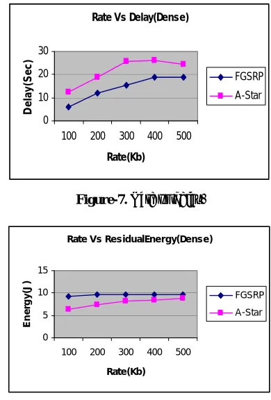
Figure-7. Shows the delay of FGSRP and A-star techniques for different rate scenario. We can conclude that the delay of our proposed FGSRP approach is 36% less than A-star approach.
Figure-8. Shows the residual energy of FGSRP and A-star techniques for different rate scenario. We can conclude that the residual energy of our proposed FGSRP approach is 18% higher than A-star approach.
4.3.2. Sparse scenario based on rate
In this experiment, we vary the rate as 100,200,300,400 and 500Kb.
Rate Vs Delay(Sparse)
0 5 10 15 20 25
100 200 300 400 500
Rate(Kb)
D
e
la
y(Se
c)
FGSRP
A-Star
Figure-9. Rate vs delay.
Rate Vs ResidualEnergy(Sparse)
0 2 4 6 8 10
100 200 300 400 500
Rate(Kb)
En
er
g
y
(J
)
FGSRP
A-Star
Figure-10. Rate vs residual energy.
Figure 9. shows the delay of FGSRP and A-star techniques for different rate scenario. We can conclude that the delay of our proposed FGSRP approach is 9% less than A-star approach.
Figure 10. shows the residual energy of FGSRP and A-star techniques for different rate scenario. We can conclude that the residual energy of our proposed FGSRP approach is 34% higher than A-star approach.
5. CONCLUSIONS
Considering the problems of Overhead of message passing, constant energy, the node cost this paper gives the solution. A-Star Algorithm consumes huge memory to keep the data of current proceeding nodes. SBGA tends to find the global optimum faster than other algorithms have a higher convergence rate. This paper proposes to develop an improved routing technique for lifetime enhancement in WSN. In fuzzy approach for estimating the node cost, the parameters link quality, energy and load.. To describe the solution in a standard
[image:6.612.84.279.261.549.2]REFERENCES
[1] Zhou. J., Mu. C. 2006. Density domination of QoS Control with localized information in wireless sensor networks. In Proceedings of the 6th International
Conference on ITS Telecommunications, pp. 21–23.
[2] Ayon Chakraborty, Kaushik Chakraborty, Swarup Kumar Mitra and M. K. Naska. 2009. “An Optimized Lifetime Enhancement Scheme for Data Gathering in Wireless Sensor Networks” Wireless Communication and senor Networks (WCSN), fifth IEEE conference at Allahabad.
[3] Pallavi D. Joshi and G. M. Asutkar. 2012. “Lifetime Enhancement of WSN by heterogeneous Power Distributions to nodes: A Design Approach” International Journal of Applied Information Systems (IJAIS) Vol. 3, No.6.
[4] Anitha, M. Selvi and Dr. N. Saravana Selvam. 2013. “Life Time Enhancement Techniques in Wireless Sensor Network: A Survey”, International Journal of Emerging Technology and Advanced Engineering. Vol 3, Issue 10.
[5] Priyanka, M. Lokhande and A. P. Thakare. 2013. “Maximization of lifetime and minimization of Delay for performance Enhancement of WSN” International Journal of technology and management Vol.2 No.1.
[6] Hadi Jamali Rad, Bahman Abolhassani and Mohammed Abdizadeh. 2010. “Lifetime Optimization via network sectoring in cooperative wireless sensor networks”, Journal of Wireless Sensor Networks, Vol. 2, No. 12, Dec.
[7] Lalit Saraswat and Dr. Sachin Kumar. 2012. “Balancing the network overload for the lifetime enhancement of wireless sensor networks”,IJESAT International Journal of engineering Science and advanced technology. Vol.2 and Issue 2.
[8] Chongmyung Park, Harksoo Kim and Inbum Jung. 2010. “Traffic-aware routing protocol for wireless sensor networks”, IEEE Inform.Sci.Appl International conference. pp 1-8.
[9] Abdul Mannan. 2012. “Self organizing Maps based Life Enhancement Framework for wireless sensor Networks”, International Arab Journal of e-technology, Vol. 2, No.4.
[10] Imad S. Alshawi, Lianshan Yan, Wei pan and Bin Luo. 2012. “Lifetime Enhancement in wireless sensor networks using Fuzzy Approach and A- star Algorithm”, IEEE sensor journal. Vol. 12 and No. 10.
[11] Vinh TRAN QUANG and Takumi MIYOSHI. 2008. “Adaptive Routing Protocol with Energy efficient and event clustering for wireless sensor networks”, IEICE transactions. Vol. E 91-B, No 9.