https://doi.org/10.5194/hess-22-5759-2018 © Author(s) 2018. This work is distributed under the Creative Commons Attribution 4.0 License.
Hybridizing Bayesian and variational data assimilation
for high-resolution hydrologic forecasting
Felipe Hernández and Xu Liang
Department of Civil and Environmental Engineering, University of Pittsburgh, Pittsburgh, PA, 15261, USA Correspondence:Xu Liang ([email protected])
Received: 18 July 2017 – Discussion started: 11 August 2017
Revised: 5 September 2018 – Accepted: 6 September 2018 – Published: 9 November 2018
Abstract.The success of real-time estimation and forecast-ing applications based on geophysical models has been pos-sible thanks to the two main existing frameworks for the determination of the models’ initial conditions: Bayesian data assimilation and variational data assimilation. However, while there have been efforts to unify these two paradigms, existing attempts struggle to fully leverage the advantages of both in order to face the challenges posed by modern high-resolution models – mainly related to model indeter-minacy and steep computational requirements. In this article we introduce a hybrid algorithm called OPTIMISTS (Opti-mized PareTo Inverse Modeling through Integrated STochas-tic Search) which is targeted at non-linear high-resolution problems and that brings together ideas from particle fil-ters (PFs), four-dimensional variational methods (4D-Var), evolutionary Pareto optimization, and kernel density estima-tion in a unique way. Streamflow forecasting experiments were conducted to test which specific configurations of OP-TIMISTS led to higher predictive accuracy. The experiments were conducted on two watersheds: the Blue River (low res-olution) using the VIC (Variable Infiltration Capacity) model and the Indiantown Run (high resolution) using the DHSVM (Distributed Hydrology Soil Vegetation Model). By selecting kernel-based non-parametric sampling, non-sequential eval-uation of candidate particles, and through the multi-objective minimization of departures from the streamflow observations and from the background states, OPTIMISTS was shown to efficiently produce probabilistic forecasts with comparable accuracy to that obtained from using a particle filter. More-over, the experiments demonstrated that OPTIMISTS scales well in high-resolution cases without imposing a significant computational overhead. With the combined advantages of allowing for fast, non-Gaussian, non-linear, high-resolution
prediction, the algorithm shows the potential to increase the efficiency of operational prediction systems.
1 Introduction
overfit-ting is a much bigger threat due to the phenomenon of equi-finality (Beven, 2006).
There exists a plethora of techniques to initialize the state variables of a model through the incorporation of avail-able observations, and they possess overlapping features that make it difficult to develop clear-cut classifications. How-ever, two main schools can be fairly identified: Bayesian data assimilation and variational data assimilation. Bayesian data assimilation creates probabilistic estimates of the state vari-ables in an attempt to also capture their uncertainty. These state probability distributions are adjusted sequentially to better match the observations using Bayes’ theorem. While the Kalman filter (KF) is constrained to linear dynamics and Gaussian distributions, ensemble Kalman filters (EnKF) can support non-linear models (Evensen, 2009), and particle fil-ters (PFs) can also manage non-Gaussian estimates for added accuracy (Smith et al., 2013). The stochastic nature of these Bayesian filters is highly valuable because equifinality can rarely be avoided and because of the benefits of quantifying uncertainty in forecasting applications (Verkade and Werner, 2011; Zhu et al., 2002). While superior in accuracy, PFs are usually regarded as impractical for high-dimensional appli-cations (Snyder et al., 2008), and thus recent research has focused on improving their efficiency (van Leeuwen, 2015). On the other hand, variational data assimilation is more akin to traditional calibration approaches (Efstratiadis and Koutsoyiannis, 2010) because of its use of optimization methods. It seeks to find a single–deterministic initial-state-variable combination that minimizes the departures (or varia-tions) of the modelled values from the observations (Reichle et al., 2001) and, commonly, from their history. One- to three-dimensional variants are also employed sequentially, but the paradigm lends itself easily to evaluating the performance of candidate solutions throughout an extended time window in four-dimensional versions (4D-Var). If the model’s dynamics are linearized, the optimum can be very efficiently found in the resulting convex search space through the use of gradient methods. While this feature has made 4D-Var very popular in meteorology and oceanography (Ghil and Malanotte-Rizzoli, 1991), its application in hydrology has been less widespread because of the difficulty of linearizing land-surface physics (Liu and Gupta, 2007). Moreover, variational data assimila-tion requires the inclusion of computaassimila-tionally expensive ad-joint models if one wishes to account for the uncertainty of the state estimates (Errico, 1997).
Traditional implementations from both schools have in-teresting characteristics and thus the development of hy-brid methods has received considerable attention (Bannis-ter, 2016). For example, Bayesian filters have been used as adjoints in 4D-Var to enable probabilistic estimates (Zhang et al., 2009). Moreover, some Bayesian approaches have been coupled with optimization techniques to select ensem-ble members (Dumedah and Coulibaly, 2013; Park et al., 2009). The fully hybridized algorithm 4DEnVar (Buehner et al., 2010) is gaining increasing attention for weather
predic-tion (Desroziers et al., 2014; Lorenc et al., 2015). It is es-pecially interesting that some algorithms have defied the tra-ditional choice between sequential and extended-time eval-uations. Weakly constrained 4D-Var allows state estimates to be determined at several time steps within the assimilation time window and not only at the beginning (Ning et al., 2014; Trémolet, 2006). Conversely, modifications to EnKFs and PFs have been proposed to extend the analysis of candidate members/particles to span multiple time steps (Evensen and van Leeuwen, 2000; Noh et al., 2011). The success of these hybrids demonstrates that there is a balance to be sought be-tween the allowed number of degrees of freedom and the amount of information to be assimilated at once.
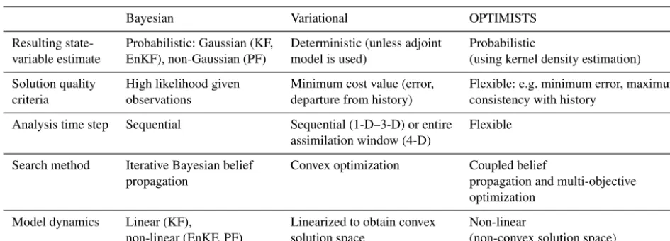
Following these promising paths, in this article we in-troduce OPTIMISTS (Optimized PareTo Inverse Modelling through Integrated STochastic Search), a hybrid data as-similation algorithm whose design was guided by the two stated goals: (i) to allow for practical scalability to high-dimensional models and (ii) to enable balancing the imper-fect observations and the imperimper-fect model estimates to min-imize overfitting. Table 1 summarizes the main characteris-tics of typical Bayesian and variational approaches and their contrasts with those of OPTIMISTS. Our algorithm incorpo-rates the features that the literature has found to be the most valuable from both Bayesian and variational methods while mitigating the deficiencies or disadvantages associated with these original approaches (e.g. the linearity and determinism of 4D-Var and the limited scalability of PFs): Non-Gaussian probabilistic estimation and support for non-linear model dy-namics have been long held as advantageous over their alter-natives (Gordon et al., 1993; van Leeuwen, 2009) and, simi-larly, meteorologists favour extended-period evaluations over sequential ones (Gauthier et al., 2007; Rawlins et al., 2007; Yang et al., 2009). As shown in the table, OPTIMISTS can readily adopt these proven strategies.
Table 1.Comparison between the main features of standard Bayesian data assimilation algorithms (KF: Kalman filter, EnKF: ensemble KF, PF: particle filter), variational data assimilation (one- to four-dimensional), and OPTIMISTS.
Bayesian Variational OPTIMISTS
Resulting state- Probabilistic: Gaussian (KF, Deterministic (unless adjoint Probabilistic
variable estimate EnKF), non-Gaussian (PF) model is used) (using kernel density estimation)
Solution quality High likelihood given Minimum cost value (error, Flexible: e.g. minimum error, maximum criteria observations departure from history) consistency with history
Analysis time step Sequential Sequential (1-D–3-D) or entire Flexible assimilation window (4-D)
Search method Iterative Bayesian belief Convex optimization Coupled belief
propagation propagation and multi-objective
optimization
Model dynamics Linear (KF), Linearized to obtain convex Non-linear
non-linear (EnKF, PF) solution space (non-convex solution space)
2 Data assimilation algorithm
In this section we describe OPTIMISTS, our proposed data assimilation algorithm which combines advantageous fea-tures from several Bayesian and variational methods. As will be explained in detail for each of the steps of the algorithm, these features were selected with the intent of mitigating the limitations of existing methods. OPTIMISTS allows select-ing a flexible data assimilation time step 1t – i.e. the time window in which candidate state configurations are com-pared to observations. It can be as short as the model time step or as long as the entire assimilation window. For each assimilation time step at timeta new state probability distri-bution St+1t is estimated from the current distributionSt, the model, and one or more observations otobs:t+1t. For hy-drologic applications, as those explored in this article, these states Sinclude land-surface variables within the modelled watershed such as soil moisture, snow cover and water equiv-alent, and stream water volume; and observationsoare typ-ically of streamflow at the outlet (Clark et al., 2008), soil moisture (Houser et al., 1998), and/or snow cover (Andreadis and Lettenmaier, 2006). However, the description of the al-gorithm will use field-agnostic terminology to not discourage its application in other disciplines.
State probability distributionsSin OPTIMISTS are deter-mined from a set of weighted root or base sample statessi
using multivariate weighted kernel density estimation (West, 1993). This form of non-parametric distributions stands in stark contrast with those from KFs and EnKFs in their ability to model non-Gaussian behaviour – an established advantage of PFs. Each of these samples or ensemble members si is
comprised of a value vector for the state variables. The ob-jective of the algorithm is then to produce a set ofnsamples sti+1t with corresponding weightswi for the next
assimila-tion time step to determine the target distribuassimila-tionSt+1t.
This process is repeated iteratively each assimilation time step1t until the entire assimilation time frame is covered, at which point the resulting distribution can be used to per-form the forecast simulations. In Sect. 2.1 we describe the main ideas and steps involved in the OPTIMISTS data as-similation algorithm; details regarding the state probability distributions, mainly on how to generate random samples and evaluate the likelihood of particles, are explained in Sect. 2.2; and modifications required for high-dimensional problems are described in Sect. 2.3.
2.1 Description of the OPTIMISTS data assimilation algorithm
Let a “particle”Pi be defined by a “source” (or initial)
vec-tor of state variables sti (which is a sample of distribution St), a corresponding “target” (or final) state vectorsti+1t (a sample of distributionSt+1t), a set of output valuesoti:t+1t (those that have corresponding observationsotobs:t+1t), a set of fitness metricsfi, a rankri, and a weightwi. Note that the
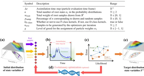
denomination “particle” stems from the PF literature and is analogous to the “member” term in EnKFs. The fitness met-ricsfi are used to compare particles with each other in the light of one or more optimization objectives. The algorithm consists of the following steps, whose motivation and details are included in the sub-subsections below and their interac-tions illustrated in Fig. 1. Table 2 lists the meaning of each of the seven global parameters (1t,n,wroot,psamp,kF-class,
nevo, andg).
1. Drawing: draw root samplessti fromSt in descending weight order untilP
wi≥wroot.
Table 2.List of global parameters in OPTIMISTS.
Symbol Description Range
1t Assimilation time step (particle evaluation time frame) R+
n Total number of root statessi in the probability distributions N≥2
wroot Total weight of root samples drawn fromSt R∈ [0,1] psamp Percentage ofncorresponding to drawn and random samples R∈ [0,1]
kF-class Whether or not to use F-class kernels. If not, use D-class kernels. true or false
nevo Samples to be generated by the optimizers per iteration N≥2
g Level of greed for the assignment of particle weightswi R∈ [−1,1]
Figure 1.Steps in OPTIMISTS, to be repeated for each assimilation time step1t. In this example state vectors have two variables, obser-vations are of streamflow, and particles are judged using two user-selected objectives: the likelihood givenStto be maximized and the error given the observations to be minimized.(a)Initial state kernel density distributionSt from which root samples (purple rhombi) are taken during the drawing step and random samples (yellow rhombi) are taken during the sampling step.(b)Execution of the model (simulation step) for each source sample for a time equal to1t to compute output variables (for comparison with observations) and target samples (circles).(c)Evaluation of each particle (evaluation step) based on the objectives and organization into non-domination fronts (ranking step). The dashed lines represent the fronts while the arrows denote domination relationships between particles in adjacent fronts.(d)Optional optimization step which can be executed several times and that uses a population-based evolutionary optimization algorithm to generate additional samples (red rhombi).(e)Target state kernel density distributionSt+tconstructed from the particles’ final samples (circles) after being weighted according to the rank of their front (weighting step): kernels centred on samples with higher weight (shown larger) have a higher probability density contribution.
3. Simulation: computesti+1t andoti:t+1t from each non-evaluated samplesti using the model.
4. Evaluation: compute the fitness valuesfi for each par-ticlePi.
5. Optimization: create additional samples using evolu-tionary algorithms and return to 3 (if number of samples is belown).
6. Ranking: assign ranksri to all particlesPi using
non-dominated sorting.
7. Weighting: compute the weightwi for each particlePi
based on its rankri.
2.1.1 Drawing step
While traditional PFs draw all the root (or base) samples fromSt (Gordon et al., 1993), OPTIMISTS can limit this se-lection to a subset of them. The root samples with the highest
weight – those that are the best performers – are drawn first, followed by the next ones in descending weight order, until the total weight of the drawn samplesPw
i reacheswroot.
wroot thus controls what percentage of the root samples to draw, and, if set to one, all of them are selected.
2.1.2 Sampling step
(Liu and Chen, 1998). The parameter wroot therefore con-trols the intensity with which this feature is applied to offer users some level of flexibility. Generating random samples at the beginning, instead of resampling those that have been already evaluated, could lead to discarding degenerate parti-cles (those with high errors) early on and contribute to im-proved efficiency, given that the ones discarded are mainly those with the lowest weight as determined in the previous assimilation time step.
2.1.3 Simulation step
In this step, the algorithm uses the model to compute the re-sulting state vectorsti+1tand an additional set of output vari-ablesoti:t+1t for each of the samples (it is possible that state variables double as output variables). The simulation is ex-ecuted starting at timet for the duration of the assimilation time step1t (not to be confused with the model time step which is usually shorter). Depending on the complexity of the model, the simulation step can be the one with the high-est computational requirements. In those cases, paralleliza-tion of the simulaparalleliza-tions would greatly help in reducing the total footprint of the assimilation process. The construction of each particlePiis started by assembling the corresponding
values computed so far:sti(drawing, sampling, and optimiza-tion steps), andsti+1t andoti:t+1t (simulation step).
2.1.4 Evaluation step
In order to determine which initial state sti is the most de-sirable, a two-term cost functionJ is typically used in vari-ational methods that simultaneously measures the resulting deviations of modelled valuesoti:t+1t from observed values otobs:t+1t and the departures from the background state distri-butionSt (Fisher, 2003). The function usually has the form shown in Eq. (1):
Ji=c1·Jbackground sti,S t
+c2
·Jobservations
oit:t+1t,oobst:t+1t, (1) wherec1andc2 are balancing constants usually set so that
c1=c2. Such a multi-criteria evaluation is crucial both to guarantee a good level of fit with the observations (sec-ond term) and to avoid the optimization algorithm to pro-duce an initial state that is inconsistent with previous states (first term) – which could potentially result in overfitting problems rooted in disproportionate violations of mass and energy conservation laws (e.g. in hydrologic applications a sharp, unrealistic rise in the initial soil moisture could re-duceJobservationsbut would increaseJbackground). In Bayesian methods, since the consistency with the state history is main-tained by sampling only from the prior or background dis-tributionSt, single-term functions are used instead – which typically measure the probability density or likelihood of the modelled values given a distribution of the observations.
In OPTIMISTS any such fitness metric could be used and, most importantly, the algorithm allows defining several of them. Moreover, users can determine whether each function is to be minimized (e.g. costs or errors) or maximized (e.g. likelihoods). We expect these features to be helpful if one wishes to separate errors when multiple types of observations are available (Montzka et al., 2012) and as a more natural way to consider different fitness criteria (lumping them to-gether in a single function as in Eq. (1) can lead to balancing and “apples and oranges” complications). Moreover, it might prove beneficial to take into account the consistency with the state history both by explicitly defining such an objective here and by allowing states to be sampled from the previ-ous distribution (and thus compounding the individual mech-anisms of Bayesian and variational methods). Functions to measure this consistency are proposed in Sect. 2.2. With the set of objective functions defined by the user, the algorithm computes the vector of fitness metricsfi for each particle during the evaluation step.
2.1.5 Optimization step
The optimization step is optional and is used to generate ad-ditional particles by exploiting the knowledge encoded in the fitness values of the current particle ensemble. In a twist to the signature characteristic of variational data assimilation, OPTIMISTS incorporates evolutionary multi-objective opti-mization algorithms (Deb, 2014) instead of the established gradient-based, single-objective methods. Evolutionary opti-mizers compensate for their slower convergence speed with the capability of efficiently navigating non-convex solution spaces (i.e. the models and the fitness functions do not need to be linear with respect to the observations and the states). This feature effectively opens the door for variational meth-ods to be used in disciplines where the linearization of the driving dynamics is either impractical, inconvenient, or un-desirable. Whereas any traditional multi-objective global op-timization method would work, our implementation of OP-TIMISTS features a state-of-the-art adaptive ensemble algo-rithm similar to the algoalgo-rithm of Vrugt and Robinson (2007), AMALGAM, that allows model simulations to be run in par-allel (Crainic and Toulouse, 2010). The optimizer ensemble includes a genetic algorithm (Deb et al., 2002) and a hybrid approach that combines ant colony optimization (Socha and Dorigo, 2008) and Metropolis–Hastings sampling (Haario et al., 2001).
deter-mine what percentage of the particles is generated in which way. For example, for relatively small values ofwrootand a
psampof 0.2, 80 % of the particles will be generated by the optimization algorithms. In this way, OPTIMISTS offers its users the flexibility to behave anywhere in the range between fully Bayesian (psamp=1) and fully variational (psamp=0) in terms of particle generation. In the latter case, in which no root and random samples are available, the initial population or ensemble of statesstiis sampled uniformly from the viable range of each state variable.
2.1.6 Ranking step
A fundamental aspect of OPTIMISTS is the way in which it provides a probabilistic interpretation to the results of the multi-objective evaluation, thus bridging the gap between Bayesian and variational assimilation. Such method has been used before (Dumedah et al., 2011) and is based on the employment of non-dominated sorting (Deb, 2014), another technique from the multi-objective optimization literature, which is used to balance the potential tensions between var-ious objectives. This sorting approach is centred on the con-cept of dominance, instead of organizing all particles from the best to the worst. A particle dominates another if it out-performs it according to at least one of the criteria/objectives while simultaneously is not being outperformed according to any of the others. Following this principle, in the ranking step particles are grouped in fronts comprised of members which are mutually non-dominated; that is, none of them is dominated by any of the rest. Particles in a front, therefore, represent the effective trade-offs between the competing cri-teria.
Figure 1c illustrates the result of non-dominated sorting applied to nine particles being analysed under two objectives: minimum deviation from observations and maximum likeli-hood given the background state distributionSt. Note that, if a single-objective function is used, the sorting method as-signs ranks from best to worst according to that function, and two particles would only share ranks if their fitness values co-incide. In our implementation we use the fast non-dominated sorting algorithm to define the fronts and assign the corre-sponding ranks ri (Deb et al., 2002). More efficient
non-dominated sorting alternatives are available if performance becomes an issue (Zhang et al., 2015).
2.1.7 Weighting step
In this final step, OPTIMISTS assigns weights wi to each
particle according to its rankri as shown in Eqs. (2) and (3).
This Gaussian weighting depends on the ensemble sizenand the greed parametergand is similar to the one proposed by Socha and Dorigo (2008). Whengis equal to zero, particles in all fronts are weighted uniformly; whengis equal to one, only particles in the Pareto or first front are assigned non-zero weights. With this, the final estimated probability distribution
of state variables for the next time stepSt+1t can be estab-lished using multivariate weighted kernel density estimation (details in the next sub-section), as demonstrated in Fig. 1e., by taking all target statessti+1t (circles) as the centroids of the kernels. The obtained distributionSt+1t can then be used as the initial distribution for a new assimilation time step or, if the end of the assimilation window has been reached, it can be used to perform (ensemble) forecast simulations.
wi=
1
σ √
2πe −(ri−1)
2
2σ2 (2)
σ=n·h0.1+9.9·(1−g)5i (3)
2.2 Model state probability distributions
As mentioned before, OPTIMISTS uses kernel density prob-ability distributions (West, 1993) to model the stochastic es-timates of the state-variable vectors. The algorithm requires two computations related to the state-variable probability dis-tribution St: obtaining the probability density p or likeli-hoodLof a sample and generating random samples. The first computation can be used in the evaluation step as an objec-tive function to preserve the consistency of particles with the state history (e.g. to penalize aggressive departures from the prior conditions). It should be noted that several metrics that try to approximate this consistency exist, from very simple (Dumedah et al., 2011) to quite complex (Ning et al., 2014). For example, it is common in variational data assimilation to utilize the background error term
Jbackground=(s−sb)TC−1(s−sb) , (4)
wheresbandCare the mean and the covariance of the back-ground state distribution (St in our case), which is assumed to be Gaussian (Fisher, 2003). The termJbackgroundis plugged into the cost function shown in Eq. (1). For OPTIMISTS, we propose that the probability density of the weighted state ker-nel density distributionSt at a given point (p) be used as a stand-alone objective. The density is given by Eq. (5) (Wand and Jones, 1994). If Gaussian kernels are selected, the ker-nel functionK, parameterized by the bandwidth matrixB, is evaluated using Eq. (6).
p (s|s)=P1 wi
n
X
i=1
[wi·KB(s−si)] (5)
KBGauss(z)=√ 1
(2π )n· |B|exp
−1
2z
TB−1z (6)
samples si, effectively encodes the uncertainty of the state
variables. Several optimization-based methods exist to com-puteBby attempting to minimize the asymptotic mean inte-grated squared error (AMISE) (Duong and Hazelton, 2005; Sheather and Jones, 1991). However, here we opt to use a simplified approach for the sake of computational efficiency: we determineBby scaling down the sample covariance ma-trixCusing Silverman’s rule of thumb, which takes into ac-count the number of samplesnand the dimensionality of the distributiond, as shown in Eq. (7) (Silverman, 1986). Fig-ure 1 shows the density of two two-dimensional example dis-tributions using this method (Fig. 1a and e). If computational constraints are not a concern, using AMISE-based methods or kernels with variable bandwidth (Hazelton, 2003; Terrell and Scott, 1992) could result in higher accuracy.
BSilverman=
4
d+2 d+24
·n−d2+4·C (7)
Secondly, OPTIMISTS’ sampling step requires generating random samples from a multivariate weighted kernel den-sity distribution. This is achieved by dividing the problem into two: we first select the root sample and then generate a random sample from the kernel associated with that base sample. The first step corresponds to randomly sampling a multinomial distribution withncategories and assigning the normalized weights of the particles as the probability of each category. Once a root samplesrootis selected, a random sam-plesrandomcan be generated from a vectorvof independent standard normal random values of sized and a matrixAas shown in Eq. (8).Acan be computed from a Cholesky de-composition (Krishnamoorthy and Menon, 2011) such that AAT =B. Alternatively, an eigendecomposition can be used to obtainQ3QT =Bto then setA=Q312.
srandom=sroot+Av (8)
Both computations (density or likelihood and sampling) re-quireBto be invertible and, therefore, that none of the vari-ables have zero variance or are perfectly linearly dependent on each other. Zero-variance variables must therefore be iso-lated andBmarginalized before attempting to use Eq. (6) or to computeA. Similarly, linear dependencies must also be identified beforehand. If we include variables one by one in the construction ofC, we can determine if a newly added one is linearly dependent if the determinant of the extended sam-ple covariance matrixCis zero. Once identified, the regres-sion coefficients for the dependent variable can be efficiently computed fromCfollowing the method described by Fried-man et al. (2008). The constant coefficient of the regression must also be calculated for future reference. What this pro-cess effectively does is to determine a linear model for each dependent variable that is represented by a set of regression coefficients. Dependent variables are not included inC, but they need to be taken into account afterwards (e.g. by
deter-mining their values for the random samples by solving the linear model with the values obtained for the variables inC).
2.3 High-dimensional state vectors
When the state vector of the model becomes large (i.e.d in-creases), as is the case for distributed high-resolution numer-ical models, difficulties start to arise when dealing with the computations involving the probability distribution. At first, the probability density, as computed with Eqs. (5) and (6), tends to diverge either towards zero or towards infinity. This phenomenon is related to the normalization of the density – so that it can integrate to one – and to its fast exponential de-cay as a function of the sample’s distance from the kernel’s centres. In these cases we propose replacing the density com-putation with an approximated likelihood formulation that is proportional to the inverse square Mahalanobis distance (Mahalanobis, 1936) to the root samples, thus skipping the exponentiation and normalization operations of the Gaussian density. This simplification, which corresponds to the inverse square difference between the sample value and the kernel’s mean in the univariate case, is shown in Eq. (9). The result-ing distortion of the Gaussian bell-curve shape does not af-fect the results significantly, given that OPTIMISTS uses the fitness functions only to check for domination between parti-cles – so only the signs of the differences between likelihood values are important and not their actual magnitudes.
LMahalanobis(s|S)= 1
P
wi n
X
i=1
wi
(s−si)TB−1(s−si)
(9)
However, computational constraints might also make this simplified approach unfeasible both due to theO(d2)space requirements for storing the bandwidth matrix B and the
O(d3) time complexity of the decomposition algorithms, which rapidly become huge burdens for the memory and the processors. Therefore, we can chose to sacrifice some accu-racy by using a diagonal bandwidth matrix B which does not include any covariance term – only the variance terms in the diagonal are computed and stored. This implies that, even though the multiplicity of root samples would help in maintaining a large portion of the covariance, another por-tion is lost by preventing the kernels from reflecting the exist-ing correlations. In other words, variables would not be ren-dered completely independent, but rather conditionally inde-pendent because the kernels are still centred on the set of root samples. Kernels using diagonal bandwidth matrices are referred to as “D-class” kernels while those using the full covariance matrix are referred to as “F-class” kernels. The
kF-classparameter controls which version is used.
With only the diagonal terms of matrixBavailable (bjj),
each variablej, as shown in Eq. (10):
Lindependent(s|S)= 1 d
√
2πP
wi d
X
j=1
n
X
i=1 (
wi·exp
"
− sj−si,j
2
2bjj
#)
, (10)
where sj represents the jth element of state vector s and
si,j represents the jth element of theith sample of
proba-bility distributionS. Independent and marginal random sam-pling of each variable can also be applied to replace Eq. (8) by adding random Gaussian residuals to the elements of the selected root samplesroot. Sparse bandwidth matrices (Fried-man et al., 2008; Ghil and Malanotte-Rizzoli, 1991) or low-rank approximations (Bannister, 2008; Ghorbanidehno et al., 2015; Li et al., 2015) could be worthwhile intermediate al-ternatives to our proposed quasi-independent approach to be explored in the future.
3 Experimental set-up
In this section we prepare the elements to investigate whether OPTIMISTS can help improve the forecasting skill of hy-drologic models. More specifically, the experiments seek to answer the following questions. Which characteristics of Bayesian and variational methods are the most advanta-geous? How can OPTIMISTS be configured to take advan-tage of these characteristics? How does the algorithm com-pare to established data assimilation methods? And how does it perform with high-dimensional applications? To help an-swer these questions, this section first introduces two case studies and then it describes a traditional PF that was used for comparison purposes.
3.1 Case studies
We coupled a Java implementation of OPTIMISTS with two popular open-source distributed hydrologic modelling engines: Variable Infiltration Capacity (VIC) (Liang et al., 1994, 1996a b; Liang and Xie, 2001, 2003) and the Dis-tributed Hydrology Soil Vegetation Model (DHSVM) (Wig-mosta et al., 1994, 2002). VIC is targeted at large water-sheds by focusing on vertical subsurface dynamics and also enabling intra-cell precipitation, soil, and vegetation hetero-geneity. The DHSVM, on the other hand, was conceived for high-resolution representations of the Earth’s surface, allow-ing for saturated and unsaturated subsurface flow routallow-ing and 1-D or 2-D surface routing (Zhang et al., 2018). Both engines needed several modifications so that they could be executed in a non-continuous fashion as required for sequential assim-ilation. Given the non-Markovian nature of surface routing schemes coupled with VIC that are based either on multi-scale approaches (Guo et al., 2004; Wen et al., 2012) or on
the unit hydrograph concept (Lohmann et al., 1998), a sim-plified routing routine was developed that treats the model cells as channels – albeit with longer retention times. In the simplified method, direct run-off and baseflow produced by each model cell is partly routed through an assumed equiva-lent channel (slow component) and partly poured directly to the channel network (fast component). Both the channel net-work and the equivalent channels representing overland flow hydraulics are modelled using the Muskingum method. On the other hand, several important bugs in version 3.2.1 of the DHSVM, mostly related to the initialization of state variables but also pertaining to routing data and physics, were fixed.
We selected two watersheds to perform streamflow fore-casting tests using OPTIMISTS: one with the VIC model running at a 1/8◦resolution for the Blue River in Oklahoma and the other with the DHSVM running at a 100 m resolu-tion for the Indiantown Run in Pennsylvania. Table 3 lists the main characteristics of the two test watersheds and the information of their associated model configurations. Fig-ure 2 shows the land cover map together with the layout of the modelling cells for the two watersheds. The multi-objective ensemble optimization algorithm included in OP-TIMISTS was employed to calibrate the parameters of the two models with the streamflow measurements from the cor-responding USGS stations. For the Blue River, the traditional
`2-norm Nash–Sutcliffe efficiency (NSE`2) (which focuses
mostly on the peaks of hydrographs), an `1-norm version of the Nash–Sutcliffe efficiency coefficient (NSE`1) (Krause
et al., 2005), and the mean absolute relative error (MARE) (which focuses mostly on the inter-peak periods) were used as optimization criteria. From 85 600 candidate parameteri-zations tried, one was chosen from the resulting Pareto front with NSE`2=0.69, NSE`1=0.56, and MARE=44.71 %.
For the Indiantown Run, the NSE`2, MARE, and absolute
bias were optimized, resulting in a parameterization, out of 2575, with NSE`2=0.81, MARE=37.85 %, and an
ab-solute bias of 11.83 L s−1.
These optimal parameter sets, together with additional sets produced in the optimization process, were used to run the models and determine a set of time-lagged state-variable vec-torssto construct the state probability distributionS0at the beginning of each of a set of data assimilation scenarios. The state variables include liquid and solid interception; ponding, water equivalent, and temperature of the snow packs; and moisture and temperature of each of the soil layers. While we do not expect all of these variables to be identifiable and sensitive within the assimilation problem, we decided to be thorough in their inclusion – a decision that also increases the challenge for the algorithm in terms of the potential for over-fitting. The Blue River model application has 20 cells, with a maximum of seven intra-cell soil–vegetation partitions. After adding the stream network variables, the model has a total of
Table 3.Characteristics of the two test watersheds: Blue River and Indiantown Run. US hydrologic units are defined in Seaber et al. (1987). Elevation information was obtained from the Shuttle Radar Topography Mission (Rodríguez et al., 2006); land cover and impervious per-centage from the National Land Cover Database, NLCD (Homer et al., 2012); soil type from CONUS-SOIL (Miller and White, 1998); and precipitation, evapotranspiration, and temperature from NLDAS-2 (Cosgrove et al., 2003). The streamflow and temperature include their range of variation of 90 % of the time (5 % tails at the high and low end are excluded).
Model characteristic Blue River Indiantown Run
USGS station; US hydrologic unit 07332500; 11140102 01572950; 02050305 Area (km2); impervious 3031; 8.05 % 14.78; 0.83 % Elevation range; average slope 158–403 m; 3.5 % 153–412 m; 14.5 % Land cover 43 % grassland, 28 % forest, 74.6 % deciduous forest
21 % pasture/hay
Soil type Clay loam (26.4 %), clay (24.8 %), Silt loam (51 %), sandy loam (49 %) sandy loam (20.26 %)
Average streamflow (90 % range) 9.06 m3s−1(0.59–44.71 m3s−1) 0.3 m3s−1(0.035–0.793 m3s−1) Average precipitation; average ET 1086; 748 mm yr−1 1176; 528 mm yr−1
Average temperature (90 % range) 17.26◦C (2.5–31◦C) 10.9◦C (−3.5–24◦C) Model cells; stream segments;d 20; 14; 812 1472; 21; 33 455
Resolution 0.125◦; daily 100 m; hourly
Calibration 167 parameters; 85 months; 18 parameters; 20 months; objectives: objectives: NSE`2, NSE`1, MARE NSE`2, MARE, absolute bias
Figure 2.Maps of the two test watersheds in the United States displaying the 30 m resolution land cover distribution from the NLCD (Homer et al., 2012).(a)Oklahoma’s Blue River watershed 0.125◦resolution VIC model application (20 cells).(b)Pennsylvania’s Indiantown Run watershed 100 m resolution DHSVM model application (1472 cells).
Three diverse scenarios were selected for the Blue River, each of them comprised of a 2-week assimilation period (when streamflow observations are assimilated) and a 2-week forecasting period (when the model is run in an open loop us-ing the states obtained at the end of the assimilation period): Scenario 1, starting on 15 October 1996, is rainy through the
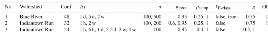
Table 4.Set-up of the three factorial experiments, including the watershed, the total number of configurations (conf.), the values assigned to OPTIMISTS’ parameters, and which objectives (objs.) were used (one objective: minimize MAE given the streamflow observations; two objectives: minimize MAE and maximize likelihood given the source or background state distributionSt).nevowas set to 25 in all cases. The total number of configurations results from combining all the possible parameter assignments listed for each experiment. Note that for Experiment 3 there are configurations that require a 4-week assimilation period (all others have a length of 2 weeks).
No. Watershed Conf. 1t n wroot psamp kF-class g Objs.
1 Blue River 48 1 d, 5 d, 2 w 100, 500 0.95 0.25, 1 false, true 0.75 1, 2 2 Indiantown Run 32 1 h, 2 w 100, 200 0.6, 0.95 0.25, 1 false 0.75 1, 2 3 Indiantown Run 24 1 h, 6 h, 1 d, 3.5 d, 2 w, 4 w 100 0.95 0.4, 1 false 0.5, 1 2
Indiantown Run, one starting on 26 July 2009 and the other on 26 August 2009.
We used factorial experiments (Montgomery, 2012) to test different configurations of OPTIMISTS on each of these sce-narios, by first assimilating the streamflow and then measur-ing the forecastmeasur-ing skill. In this type of experimental designs a set of assignments is established for each parameter and then all possible assignment combinations are tried. The de-sign allows us to establish the statistical de-significance of al-tering several parameters simultaneously, providing an ade-quate framework for determining, for example, whether us-ing a short or a long assimilation time step1t is preferable, or if utilizing the optional optimization step within the al-gorithm is worthwhile. Table 4 shows the set-up of each of the three full factorial experiments we conducted, together with the selected set of assignments for OPTIMISTS’ param-eters. The forecasts were produced in an ensemble fashion, by running the models using each of the samplessi from the
state distributionSat the end of the assimilation time period, and then using the samples’ weightswi to produce an
aver-age forecast. Deterministic model parameters (those from the calibrated models) and forcings were used in all simulations. Observation errors are usually taken into account in tradi-tional assimilation algorithms by assuming a probability dis-tribution for the observations at each time step and then per-forming a probabilistic evaluation of the predicted value of each particle/member against that distribution. As mentioned in Sect. 2, such a fitness metric, like the likelihood utilized in PFs to weight candidate particles, is perfectly compatible with OPTIMISTS. However, since it is difficult to estimate the magnitude of the observation error in general, and fitness metricsfi here are only used to determine (non-)dominance between particles, we opted to use the mean absolute er-ror (MAE) with respect to the streamflow observations in all cases.
For the Blue River scenarios, a secondary likelihood ob-jective or metric was used in some cases to select for par-ticles with higher consistency with the state history. It was computed using either Eq. (10) if kF-class was set to false or Eq. (9) if it was set to true. Equation (10) was used for all Indiantown Run scenarios given the large number of di-mensions. The assimilation period was of 2 weeks for most
configurations, except for those in Experiment 3, which have
1t=4 weeks. During both the assimilation and the fore-casting periods we used unaltered streamflow data from the USGS and forcing data from the North American Land Data Assimilation System (NLDAS-2) (Cosgrove et al., 2003) – even though a forecasted forcing would be used instead in an operational setting (e.g. from systems like NAM, Rogers et al., 2009; or ECMWF, Molteni et al., 1996). While adopting perfect forcings for the forecast period leads to an overesti-mation of their accuracy, any comparisons with control runs or between methods are still valid as they all share the same benefit. Also, removing the uncertainty in the meteorologi-cal forcings allows the analysis to focus on the uncertainty corresponding to the land surface.
3.2 Data assimilation method comparison
Comparing the performance of different configurations of OPTIMISTS can shed light into the adequacy of individ-ual strategies utilized by traditional Bayesian and variational methods. For example, producing all particles with the opti-mization algorithms (psamp=0), setting long values for1t, and utilizing a traditional two-term cost function as that in Eq. (1) makes the method behave somewhat as a strongly constrained 4D-Var approach, while sampling all particles from the source state distribution (psamp=1), setting 1t equal to the model time step, and using a single likelihood objective involving the observation error would resemble a PF. Herein we also compare OPTIMISTS with a tradi-tional PF on both model applications. Since the forcing is assumed to be deterministic, the implemented PF uses Gaus-sian perturbation of resampled particles to avoid degener-ation (Pham, 2001). Resampling is executed such that the probability of duplicating a particle is proportional to their weight (Moradkhani et al., 2012).
stream-flow observations for the assimilation time step of each al-gorithm (daily for the PF). The assimilation is performed cumulatively, meaning that the initial state distribution St was produced by assimilating all the records available since the beginning of the experiment until timet. The forecasted streamflow series are then compared to the actual measure-ments to evaluate their quality using deterministic metrics (NSE`2, NSE`1, and MARE) and two probabilistic ones: the
ensemble-based continuous ranked probability score (CRPS) (Bröcker, 2012), which is computed for each time step and then averaged for the entire duration of the forecast; and the average normalized probability density p of the observed streamflow qobs given the distribution of the forecasted en-sembleqforecast,
p qobs|qforecast
=
n
P
i=1
wi· 2π b2
−2
·exp
−(qobs−qi)2/ 2b2 n
P
i=1
wi
, (11)
where the forecasted streamflowqforecastis composed of val-uesqi for each particleiand accompanying weightwi, and
b is the bandwidth of the univariate kernel density estimate. The bandwidth b can be obtained by utilizing Silverman’s rule of thumb (Silverman, 1986). The probabilitypis com-puted every time step, then normalized by multiplying by the standard deviation of the estimate, and then averaged for all time steps. As opposed to the CRPS, which can only give an idea of the bias of the estimate, the density pcan detect both bias and under- or overconfidence: high values for the density indicate that the ensemble is producing narrow esti-mates around the true value, while low values indicate either that the stochastic estimate is spread too thin or is centred far away from the true value.
4 Results and discussion
This section summarizes the forecasting results obtained from the three scenario-based experiments and the continu-ous forecasting experiments on the Blue River and the In-diantown Run model applications. The scenario-based ex-periments were performed to explore the effects of multiple parameterizations of OPTIMISTS, and the performance was analysed as follows. The model was run for the duration of the forecast period (2 weeks) using the state configuration encoded in each root state si of the distributionSobtained
at the end of the assimilation period for each configuration of OPTIMISTS and each scenario. We then computed the mean streamflow time series for each case by averaging the model results for each particlePi (the average was weighted
based on the corresponding weightswi). With this averaged
streamflow series, we compute the three performance metrics – the NSE`2, the NSE`1, and the MARE – based on the
ob-servations from the corresponding stream gauge. The values
for each experiment, scenario, and configuration are listed in tables in the Supplement. With these, we compute the change in the forecast performance between each configuration and a control open-loop model run (one without the benefit of assimilating the observations).
4.1 Blue River – low-resolution application
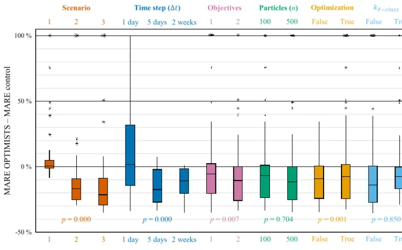
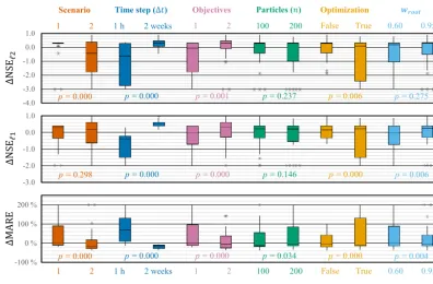
The Supplement includes the performance metrics for all the tested configurations on all scenarios and for all scenario-based experiments. Figure 3 summarizes the results for Ex-periment 1 with the VIC model application for the Blue River watershed, in which the distributions of the changes in MARE after marginalizing the results for each scenario and each of the parameter assignments are shown. That is, each box (and pair of whiskers) represents the distribution of change in MARE of all cases in the specified scenario or for which the specified parameter assignment was used. Nega-tive values in the vertical axis indicate that OPTIMISTS de-creased the error, while positive values indicate it inde-creased the error. It can be seen that, on average, OPTIMISTS im-proves the precision of the forecast in most cases, except for several of the configurations in Scenario 1 (for this scenario the control already produces a good forecast) and when using an assimilation step1tof 1 day. We performed an analysis of variance (ANOVA) to determine the statistical significance of the difference found for each of the factors indicated in the horizontal axis. While Fig. 3 shows thepvalues for the main effects, the full ANOVA table for all experiments can be found in the Supplement. From the values in Fig. 3, we can conclude that the assimilation time step, the number of objectives, and the use of optimization algorithms are all sta-tistically significant. On the other hand, the number of parti-cles and the use of F-class kernels are not.
ex-Figure 3.Box plots of the changes in forecasting error (MARE) achieved while using OPTIMISTS on Experiment 1 (Blue River). Changes are relative to an open-loop control run where no assimilation was performed. Each column corresponds to the distribution of the error changes on the specified scenario or assignment to the indicated parameter. Positive values indicate that OPTIMISTS increased the error, while negative values indicate it decreased the error. Outliers are noted as asterisks and values were limited to 100 %. For the one-objective case, the particles’ MAE was to be minimized; for the two-objective case, the likelihood given the background was to be maximized in addition. No optimization (“false”) corresponds topsamp=1.0 (i.e. all samples are obtained from the prior distribution); “true” corresponds topsamp=0.25. Thepvalues were determined using ANOVA (Montgomery, 2012) and indicate the probability that the differences in means corresponding to boxes of the same colour are produced by chance (e.g. values close to zero indicate certainty that the parameter effectively affects the forecast error).
tent is of paramount importance, perhaps to the point where the strategies used in Bayesian filters and variational meth-ods are insufficient in isolation. Indeed, the best performance was observed only when both sampling was limited to gener-ate particles from the prior stgener-ate distribution and the particles were evaluated for their consistency with that distribution.
On the other hand, we found it counterintuitive that nei-ther using a larger particle ensemble nor taking into account state-variable dependencies through the use of F-class ker-nels leads to improved results. In the first case it could be hy-pothesized that using too many particles could lead to over-fitting, since there would be more chances of particles being generated that happen to match the observations better but for the wrong reasons. In the second case, the non-parametric nature of kernel density estimation could be sufficient for en-coding the raw dependencies between variables, especially in low-resolution cases like this one, in which significant corre-lations between variables in adjacent cells are not expected to be too high. Both results deserve further investigation, es-pecially concerning the impact of D- vs. F-class kernels in high-dimensional models.
Interestingly, the ANOVA also yielded small p values for several high-order interactions (see the ANOVA table in
the Supplement). This means that, unlike the general case for factorial experiments as characterized by the sparsity-of-effects principle (Montgomery et al., 2009), specific com-binations of multiple parameters have a large effect on the forecasting skill of the model. There are significant inter-actions (with p smaller than 0.05) between the following groups of factors: objectives and 1t (p=0.001); n and
kF-class (p=0.039); 1t and the use of optimization (p= 0.000); the use of optimization andkF-class(p=0.029); the objectives,1t, and the use of optimization (p=0.043);n,
1t, andkF-class(p=0.020);n, the use of optimization, and
kF-class (p=0.013); andn,1t, the use of optimizers, and
kF-class(p=0.006). These interactions show that, for exam-ple, (i) using a single objective is especially inadequate when the time step is 1 day or when optimization is used; (ii) em-ploying optimization is only significantly detrimental when
1tis 1 day – probably because of intensified overfitting; and (iii) choosing F-class kernels leads to higher errors when1t
is small, whennis large, and when the optimizers are being used.
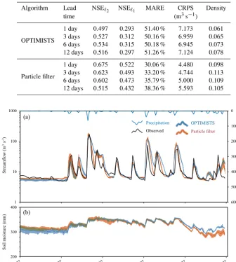
[image:12.612.104.497.67.311.2]Table 5.Continuous daily streamflow forecast performance metrics for the Blue River application using OPTIMISTS (1t=7 days; three ob-jectives: NSE`2, MARE, and likelihood;n=30; no optimization; and D-class kernels) and a traditional PF (n=30). The continuous forecast
extends from January to June 1997. The NSE`2, NSE`1, and MARE (deterministic) are computed using the mean streamflow of the forecast
ensembles and contrasting it with the daily observations, while the CRPS and the density (probabilistic) are computed taking into account all the members of the forecasted ensemble.
Algorithm Lead NSE`2 NSE`1 MARE CRPS Density
time (m3s−1)
OPTIMISTS
1 day 0.497 0.293 51.40 % 7.173 0.061 3 days 0.527 0.312 50.16 % 6.959 0.065 6 days 0.534 0.315 50.18 % 6.945 0.073 12 days 0.516 0.297 51.26 % 7.124 0.078
Particle filter
1 day 0.675 0.522 30.06 % 4.480 0.098 3 days 0.623 0.493 33.20 % 4.744 0.113 6 days 0.602 0.473 35.79 % 5.000 0.109 12 days 0.515 0.432 38.36 % 5.593 0.105
0
100
200
300
400
500
600 1
10 100 1000
P
re
ci
pi
ta
ti
on
(m
m
d
)
S
tr
ea
m
fl
ow
(
m
3s )
200 300 400
S
oil
m
oistu
re
(m
m
)
Precipitation Observed
OPTIMISTS
Particle filter
-1 -1
Figure 4.Comparison of 6-day lead time probabilistic streamflow(a)and area-averaged soil moisture(b)forecasts between OPTIMISTS (1t=7 days; three objectives: NSE`2, MARE, and likelihood;n=30; no optimization; and D-class kernels) and a traditional PF (n=30)
for the Blue River. The dark blue and orange lines indicate the mean of OPTIMISTS’ and the PF’s ensembles, respectively, while the light blue and light orange bands illustrate the spread of the forecast by highlighting the areas where the probability density of the estimate is at least 50 % of the density at the mode (the maximum) at that time step. The green bands indicate areas where the light blue and light orange bands intersect.
of around 5 days appears to be adequate for this specific model application. Also, without strong evidence for their advantages, we recommend using more particles or kernels of class F only if there is no pressure for computational fru-gality. However, the number of particles should not be too small to ensure an appropriate sample size.
Table 5 shows the results of the 5-month-long continuous forecasting experiment on the Blue River using a 30-particle PF and a configuration of OPTIMISTS with a 7-day assimi-lation time step1t, three objectives (NSE`2, MARE, and the
likelihood), 30 particles, no optimization, and D-class ker-nels. This specific configuration of OPTIMISTS was chosen from a few that were tested with the recommendations above applied. The selected configuration was the one that best bal-anced the spread and the accuracy of the ensemble as some configurations had slightly better deterministic performance but larger ensemble spread for dry weather – which lead to worse probabilistic performance.
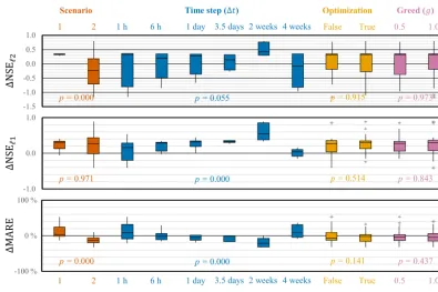
Figure 5.Box plots of the changes in forecasting performance (NSE`2, NSE`1, and MARE) achieved while using OPTIMISTS on
Experi-ment 2 (Indiantown Run). Changes are relative to an open-loop control run where no assimilation was performed. Each column corresponds to the distribution of the error metric changes on the specified scenario or assignment to the indicated parameter. Outliers are noted as stars and values were constrained to NSE`2≥ −3, NSE`1≥ −3, and MARE≤200 %. Positive values indicate improvements for the NSE`2 and the NSE`1. The meaning for the MARE and for other symbols is the same as those defined in Fig. 3.
evolution of the density, in which the mean does not nec-essarily correspond to the centre of the ensemble spread, ev-idences the non-Gaussian nature of both estimates. Both the selected configuration of OPTIMISTS and the PF methods show relatively good performance for all lead times (1, 3, 6, and 12 days) based on the performance metrics. However, the PF generally outperforms OPTIMISTS.
We offer three possible explanations for this result. First, the relatively low dimensionality of this test case does not allow OPTIMISTS to showcase its real strength, perhaps es-pecially since the large scale of the watershed does not allow for tight spatial interactions between state variables. Second, OPTIMISTS can find solutions based on multiple objectives rather than a single one, which could be advantageous when multiple types of observations are available (e.g. of stream-flow, evapotranspiration, and soil moisture). Thus, the so-lutions are likely not the best for each individual objective, but the algorithm balances their overall behaviour across the multiple objectives. Due to the lack of observations on multi-ple variables, only streamflow observations are used in these experiments even though more than one objective is used. Since it is the case that these objectives are consistent with each other, to a large extent, for the studied watershed, the strengths of using multiple objectives within the Pareto ap-proach in OPTIMISTS cannot be fully evidenced. Third,
ad-ditional efforts might be needed to find a configuration of the algorithm, together with a set of objectives, that best suits the specific conditions of the tested watershed.
While PFs remain easier to use out of the box because of their ease of configuration, the fact that adjusting the parame-ters of OPTIMISTS allowed us to trade off deterministic and probabilistic accuracy points to the adaptability potential of the algorithm. This allows for probing the spectrum between exploration and exploitation of candidate particles – which usually leads to higher and lower diversity of the ensemble, respectively.
4.2 Indiantown Run – high-resolution application
sig-Figure 6.Box plots of the changes in forecasting performance (NSE`2, NSE`1, and MARE) achieved while using OPTIMISTS on
Experi-ment 3 (Indiantown Run). Changes are relative to an open-loop control run where no assimilation was performed. Each column corresponds to the distribution of the error metric changes on the specified scenario or assignment to the indicated parameter. Positive values indicate improvements for the NSE`2and the NSE`1. See the caption of Fig. 3 for more information.
nificantly reduced the forecast skill, while the longer step al-most always improved it; and the inclusion of the secondary history-consistent objective (two objectives) also resulted in improved performance. Not only does it seem that for this watershed the secondary objective mitigated the effects of overfitting, but it was interesting to note some configurations in which using it actually helped to achieve a better fit during the assimilation period.
While the ANOVA also provided evidence against the use of optimization algorithms, we are reluctant to instantly rule them out on the grounds that there were statistically signifi-cant interactions with other parameters (see the ANOVA ta-ble in the Supplement). The optimizers led to poor results in cases with 1 h time steps or when only the first objective was used. Other statistically significant results point to the benefits of using the root samples more intensively (in oppo-sition to using random samples) and, to a lesser extent, to the benefits of maintaining an ensemble of moderate size.
Figure 6 shows the summarized changes in Experiment 3, where the effect of the time step1tis explored in greater de-tail. Once again, there appears to be evidence favouring the hypothesis that there exists a sweet spot, and in this case it ap-pears to be close to the 2-week mark: both shorter and longer time steps led to considerably poorer performance. In this experiment, with all configurations using both optimization objectives, we can see that there are no clear disadvantages
of using optimization algorithms (but also no advantages). Experiment 3 also shows that the effect of the greed parame-tergis not very significant. That is, selecting some particles from dominated fronts to construct the target state distribu-tion, and not only from the Pareto front, does not seem to affect the results.
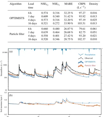
Table 6 and Fig. 7 show the results from comparing con-tinuous forecasts from the PF and from a configuration of OPTIMISTS with a time step of 1 week, two objectives, 50 particles, and no optimization. Both algorithms display overconfidence in their estimations, which is evidenced in Fig. 7 by the bias and narrowness of the ensembles’ spread. It is possible that a more realistic incorporation of uncertain-ties pertaining to model parameters and forcings (which, as mentioned, are trivialized in these tests) would help to com-pensate for overconfidence. For the time being, these exper-iments help characterize the performance of OPTIMISTS in contrast with the PF, as both algorithms are deployed under the same circumstances. In this sense, while the forecasts ob-tained using the PF show slightly better results for lead times of 6 h and 1 day, OPTIMISTS shows a better characterization of the ensemble’s uncertainty for the longer lead times.
[image:15.612.99.495.64.327.2]as-Table 6.Continuous hourly streamflow forecast performance metrics for the Indiantown Run application using OPTIMISTS (1t=7 days, two objectives,n=50, no optimization, and D-class kernels) and a traditional PF (n=50). The continuous forecast extends from September to December 2009. The NSE`2, NSE`1, and MARE (deterministic) are computed using the mean streamflow of the forecast ensembles and
contrasting it with the daily observations, while the CRPS and the density (probabilistic) are computed taking into account all the members of the forecasted ensemble.
Algorithm Lead NSE`2 NSE`1 MARE CRPS Density
time (L s−1)
OPTIMISTS
6 h 0.574 0.316 32.25 % 97.27 0.016 1 day 0.609 0.340 31.42 % 93.92 0.013 4 days 0.573 0.316 32.20 % 97.19 0.025 16 days 0.521 0.272 33.90 % 103.51 0.013
Particle filter
6 h 0.660 0.480 26.87 % 79.61 0.061 1 day 0.639 0.464 26.68 % 82.75 0.051 4 days 0.558 0.401 27.42 % 93.20 0.021 16 days 0.520 0.346 28.75 % 102.37 0.010
Figure 7.Comparison of 4-day lead time probabilistic streamflow(a)and area-averaged soil moisture(b)forecasts between OPTIMISTS (1t=7 days, two objectives,n=50, no optimization, and D-class kernels) and a traditional PF (n=50) for the Indiantown Run. The dark blue and orange lines indicate the mean of OPTIMISTS’ and the PF’s ensembles, respectively, while the light blue and light orange bands illustrate the spread of the forecast by highlighting the areas where the probability density of the estimate is at least 50 % of the density at the mode (the maximum) at that time step. The green bands indicate areas where the light blue and light orange bands intersect. Layer 2 of the soil corresponds to 100 to 250 mm depths.
similation problem increases. However, while OPTIMISTS was able to produce comparable results to those of the PF, it was not able to provide definite advantages in terms of accuracy. As suggested before, additional efforts might be needed to find the configurations of OPTIMISTS that better match the characteristics of the individual case studies and, as with the Blue River, the limitation related to the lack of ob-servations of multiple variables also applies here. Moreover, the implemented version of the PF did not present the
parti-cle degeneracy or impoverishment problems usually associ-ated with these filters when dealing with high dimensionality, which also prompts further investigation.
4.3 Computational performance
[image:16.612.132.465.127.506.2]to be generated accordingly, then accessed, and finally the result files written and accessed. This whole process takes a considerable amount of time. Therefore, everything else be-ing constant, sequential assimilation (like with PFs) automat-ically imposes additional computational requirements. In our tests we used RAM drive software to accelerate the process of running the models sequentially and, even then, the over-head imposed by OPTIMISTS was consistently below 10 % of the total computation time. Most of the computational ef-fort remained with running the model, both for VIC and the DHSVM. In this sense, model developers may consider al-lowing their engines to be able to receive input data from main memory, if possible, to facilitate data assimilation and other similar processes.
4.4 Recommendations for configuring OPTIMISTS
Finally, here we summarize the recommended choices for the parameters in OPTIMISTS based on the results of the exper-iments. In the first place, given their low observed effect, de-fault values can be used forg (around 0.5). Awroot higher than 90 % was found to be advantageous. The execution of the optimization step (psamp<1) was, on the other hand, not found to be advantageous and, therefore, we consider it a cleaner approach to simply generate all samples from the ini-tial distribution. Similarly, while not found to be disadvanta-geous, using diagonal bandwidth (D-class) kernels provide a significant improvement in computational efficiency and are thus recommended for the time being. Future work will be conducted to further explore the effect of the bandwidth con-figuration in OPTIMISTS.
Even though only two objective functions were tested, one measuring the departures from the observations being assim-ilated and another measuring the compatibility of initial sam-ples with the initial distribution, the results clearly show that it is beneficial to simultaneously evaluate candidate particles using both criteria. While traditional cost functions like the one in Eq. (1) do indeed consider both aspects, we argue that using multiple objectives has the added benefit of enriching the diversity of the particle ensemble and, ultimately, the re-sulting probabilistic estimate of the target states.
Our results demonstrated that the assimilation time step is the most sensitive parameter and, therefore, its selection must be done with the greatest involvement. Taking the re-sults together, we recommend that multiple choices be tried for any new case study looking to strike a balance between the amount of information being assimilated and the num-ber of degrees of freedom. This empirical selection should also be performed with a rough sense of what is the range of forecasting lead times that is considered the most impor-tant. Lastly, more work is required to provide guidelines to select the number of particlesnto be used. While the liter-ature suggests that more should increase forecast accuracy, our tests did not back this conclusion. We tentatively recom-mend trying different ensemble sizes based on the
computa-tional resources available and selecting the one that offers the best observed trade-off between accuracy and efficiency.
5 Conclusions and future work
In this article we introduced OPTIMISTS, a flexible, model-independent data assimilation algorithm that effectively com-bines the signature elements from Bayesian and variational methods: by employing essential features from particle fil-ters, it allows performing probabilistic non-Gaussian esti-mates of state variables through the filtering of a set of par-ticles drawn from a prior distribution to better match the available observations. Adding critical features from varia-tional methods, OPTIMISTS grants its users the option of exploring the state space using optimization techniques and evaluating candidate states through a time window of arbi-trary length. The algorithm fuses a multi-objective or Pareto analysis of candidate particles with kernel density probability distributions to effectively bridge the gap between the proba-bilistic and the variational perspectives. Moreover, the use of evolutionary optimization algorithms enables its efficient ap-plication on highly non-linear models as those usually found in most geosciences. This unique combination of features represents a clear differentiation from the existing hybrid as-similation methods in the literature (Bannister, 2016), which are limited to Gaussian distributions and linear dynamics.
We conducted a set of hydrologic forecasting factorial ex-periments on two watersheds, the Blue River with 812 state variables and the Indiantown Run with 33 455, at two dis-tinct modelling resolutions using two different modelling en-gines: VIC and the DHSVM, respectively. Capitalizing on the flexible configurations available for OPTIMISTS, these tests allowed us to determine which individual characteristics of traditional algorithms prove to be the most advantageous for forecasting applications. For example, while there is a general consensus in the literature favouring extended time steps (4-D) over sequential ones (1-D–3-D), the results from assimilating streamflow data in our experiments suggest that there is an ideal duration of the assimilation time step that is dependent on the case study under consideration, on the spatiotemporal resolution of the corresponding model appli-cation, and on the desired forecast length. Sequential time steps not only required considerably longer computational times but also produced the worst results – perhaps given the overwhelming number of degrees of freedom in contrast with the scarce observations available. Similarly, there was a drop in the performance of the forecast ensemble when the algorithm was set to use overly long time steps.