Evaluation of the Circulation Patterns in the Black Sea Using Remotely Sensed and in Situ Measurements

Evaluation of the Circulation Patterns in the Black Sea

Using Remotely Sensed and in Situ Measurements

Robert Toderascu, Eugen Rusu

Department of Applied Mechanics, “Dunarea de Jos” University of Galati, Galati, Romania Email: [email protected]

Received June 16, 2013; revised July 19, 2013; accepted August 15, 2013

Copyright © 2013 Robert Toderascu, Eugen Rusu. This is an open access article distributed under the Creative Commons Attribution License, which permits unrestricted use, distribution, and reproduction in any medium, provided the original work is properly cited.

ABSTRACT

The objective of the present work is to provide an overview of the general circulation features in the Black Sea basin. In order to achieve this, 18 years (1993-2010) of satellite data coming from the Aviso website were analyzed. A descrip-tion of the general circuladescrip-tion patterns in the Black Sea is first presented. This is followed by statistical analyses of the satellite data in 20 points covering the entire area of the sea. The reference points were chosen as follows: 12 points along the Rim cyclonic current, 3 points inside the Rim cyclonic current, 4 points on the edge of two of the biggest an-ticyclonic gyres outside the Rim current and one point in the northwestern shelf area of the basin. Rose graphics were drawn for the reference points for winter and summer time. Finally, 9 years of in situ data obtained from the Gloria

drilling platform were analyzed and compared with the satellite data. The present study shows that most of the reference points are sensitive to seasonal changes. The current velocities depend mostly on the points location: the points located on the Rim current and on the nearshore anticyclonic eddies present higher values than the ones located in or outside the general circulation features.

Keywords: Black Sea; Circulation Patterns; Statistical Analyses; Rose Graphics

1. Introduction

The Black Sea is an enclosed sea situated between Europe, Anatolia and Caucasus, bounded by the 40.56˚N and 46.33˚N latitude and 27.27˚E - 41.42˚E longitude. It is the second enclosed sea on Earth after the Caspian Sea, with a surface of 423,000 km2_{. The only connection}

bounding the Black Sea to the Global Ocean is by the Bosphorus strait, a 0.7 - 3.5 narrow channel with 31 km in length and a depth that can vary from 39 to 100 m.

The sea contains three vertical water layers that do not mix, the bottom one being the largest anoxic water body on Earth. The surface layer is located on the sea surface, spreading to 50 m depth and is the most active water layer of the sea. It responds strongly to the seasonal temperature variations and wind fields. The second layer is the cold intermediate layer located at depths that vary from 50 to 180 m. Its most significant characteristic fea-ture is the fact that the temperafea-ture here is constant, be-tween 6˚C and 8˚C, not being affected by the temperature changes in the surface layer. The cold intermediate layer is formed by the convective processes associated with the winter cooling of the surface waters [1-3]. Below the intermediate cold layer is the bottom layer where waters

are mostly stagnant showing small changes in properties, except near boundaries. In the depths higher than 1700 m, the bottom layer is subjected to geothermal heating from the sea floor, the temperature being about 8.8˚C [4]. The maximum depth of the Black Sea is of 2588 m. However, these are isolated points located in the south and south-east of the basin. The average maximum depth of the sea is 2100 m.

The Black Sea’s salinity is lower than that in the open seas or in the oceans, due to the enclosed state and high river discharges. The average salinity in the Black Sea is 18.2 PSU, but it can be much lower near the river dis-charges. The bottom layer’s salinity, however, has in-creased values by an average of 21.8 PSU. This differ-ence is maintained due to the fact that the surface and bottom waters do not mix, and the lower layer is receiv-ing more saline waters from the Mediterranean Sea. Moreover, the surface layer is exposed to rain, river dis-charges and dilution.

The cyclonic character of the Black Sea circulation resulting from the cyclonic state of the wind field pat-terns was first described by Knipovich [6] Later on Filipov [7], Boguslavskiy et al. [8], Blatov et al. [9],

provided valuable details regarding the sea circulation patterns. However, the model proposed did not contribute to a significant change to Knipovich’s classical circula-tion model.

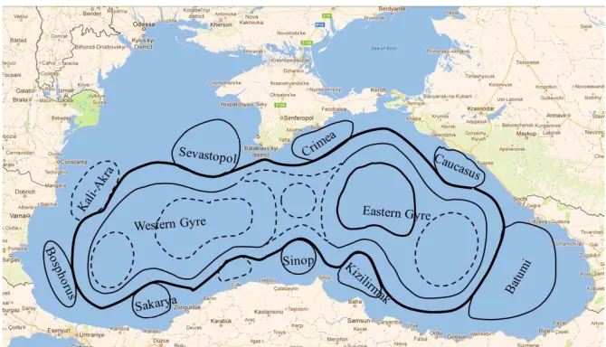
The northwestern shelf of the sea consists of a close to 200 km wide shelf that receives the fresh water input from Danube, Dniestr and Dniepr rivers. The surface circulation is characterized by a persistent cyclonic coastal current referred to as the Rim current, with a width of over 75 km and an average speed of 0.2 ms−1 _at

the surface [13]. Between the Rim current and the coast, a number of seasonal anticyclonic eddies are formed. While the Rim current meanders eastward along the Anatolian coast, it forms two anticyclonic coastal eddies that were identified and labeled by Oguz et al. [14] as the

Sinop and Kizilirmak eddies. In the eastern area of the basin, the Batumi eddy is formed. The Rim current flows along the Caucasian coast to the narrow continental slope, meandering in the form of backward curling. The jet separates three cyclonic eddies of the eastern basin that constitute the multiple cells of the Eastern Basin Cyc-lonic Gyre [13]. In the coastal side of the offshore jet, a small anticyclonic eddy is formed, called the Caucasian eddy. The Rim current continues to meander to the south of the Crimean Peninsula between two larger coastal anticyclonic eddies and two cyclonic eddies located in the central part of the basin. The anticyclonic eddies lo-cated on the northern side are referred as the Crimean Eddy and Sevastopol Eddy, respectively [13].

While it proceeds southwest towards the Bosphorus area, the Rim current creates the Bosphorus eddy. A small anticyclonic eddy is formed in the western area of the Black Sea basin, between Sevastopol and Bosphorus eddies, labeled as Kali-Akra. Its basin-wide circulation is closed with the Sakarya eddy, situated in the southwest area.

Among the above mentioned eddies, Batumi and Se-

vastopol are the most permanent and largest mesoscale structures [15,16]. Figure 1 presents a scheme of the Black Sea surface circulation as discussed above. The solid lines indicate the recurrent features of the general circulation.

2. Statistical Analysis of the Circulation

Patterns Using Satellite Data

In order to achieve a better understanding of the current fields in the Black Sea basin and of their time and space variations, 18 years of satellite data were analyzed, cov-ering the time period 1993-2010. The satellite data were obtained from Aviso website [17] and contains daily measurements of the U and V components of the currents with a spatial resolution of approximately 10 km on the horizontal and of 13 km on the vertical.

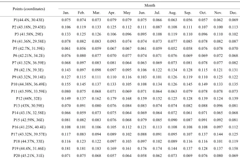
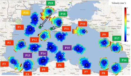
20 reference points were considered in the present analysis, as shown in Figure 2. The first 12 points (P1, P2, … P12) were considered on the Rim current (with red), points P13-P15 were located inside the Rim cyc-lonic current (with purple), points P16, P17 at the edge of the Batumi eddy, P18, P19 at the edge of the Sinop eddy (with green) and point P20 was located on the north-western shelf area of the Black Sea basin (with orange). In Table 1 the coordinates of the reference points are presented, along with the monthly averaged values of current velocities. Table 2 shows the statistical analyses for the reference points considering the following pa-rameters: minimum, maximum, mean and median values, standard deviation, skewness and kurtosis. In Table 3, percentile analyses regarding the 50th and 95th percen-tiles are presented for the reference points considered, grouped in winter and summer time, respectively where winter time is the six month period from October to March and summer from April to September.

Figure 2. The bathymetric map of the Black Sea with the location of the 20 reference points as follows: red—points located on the Rim cyclonic current, purple—points located inside the Rim current, green—points located at the edge of the anticyclonic eddies, orange—point located in the northwestern shelf area of the sea.

Table 1. Monthly averaged values of the current velocity (ms−1_{) for the reference points (P1, P2, … P20) for the period 1993-2010.}

Month Points (coordinates)

Jan. Feb. Mar. Apr. May Jun. Jul. Aug. Sep. Oct. Nov. Dec.

P1(44.4N, 30.43E) 0.075 0.074 0.073 0.079 0.079 0.075 0.066 0.063 0.056 0.057 0.062 0.069

P2 (43.18N, 29.43E) 0.106 0.119 0.133 0.125 0.112 0.111 0.087 0.108 0.111 0.107 0.100 0.113

P3 (41.58N, 29E) 0.133 0.125 0.126 0.106 0.096 0.095 0.108 0.119 0.110 0.096 0.110 0.102

P4 (41.36N, 29.58E) 0.078 0.082 0.083 0.093 0.074 0.074 0.073 0.077 0.085 0.078 0.082 0.087

P5 (42.7N, 31.59E) 0.061 0.056 0.059 0.067 0.067 0.061 0.059 0.052 0.058 0.076 0.078 0.070

P6 (42.21N, 34.2E) 0.076 0.080 0.077 0.070 0.077 0.074 0.071 0.076 0.069 0.069 0.072 0.068

P7 (41.32N, 36.59E) 0.068 0.097 0.083 0.081 0.064 0.063 0.069 0.073 0.081 0.078 0.077 0.082

P8 (42.1N, 39.3E) 0.143 0.097 0.098 0.097 0.095 0.106 0.122 0.134 0.128 0.115 0.121 0.131

P9 (43.32N, 39.14E) 0.127 0.115 0.111 0.110 0.116 0.103 0.101 0.126 0.119 0.110 0.125 0.122

P10 (44.38N, 36.49E) 0.155 0.145 0.137 0.133 0.105 0.108 0.134 0.126 0.145 0.149 0.133 0.135

P11 (43.59N, 33.59E) 0.080 0.075 0.068 0.071 0.069 0.071 0.064 0.063 0.079 0.078 0.078 0.073

P12 (44N, 32E) 0.149 0.137 0.162 0.179 0.168 0.159 0.152 0.125 0.128 0.139 0.124 0.139

P13 (43N, 30.59E) 0.070 0.091 0.080 0.076 0.084 0.083 0.074 0.074 0.082 0.088 0.096 0.081

P14 (43.1N, 32.58E) 0.066 0.059 0.073 0.075 0.064 0.069 0.064 0.072 0.061 0.071 0.065 0.068

P15 (42.59N, 36E) 0.081 0.082 0.083 0.076 0.068 0.079 0.085 0.090 0.087 0.091 0.092 0.081

P16 (41.23N, 40.4E) 0.108 0.101 0.106 0.105 0.112 0.121 0.113 0.108 0.108 0.108 0.097 0.112

P17 (43.32N, 39.57E) 0.117 0.083 0.094 0.089 0.102 0.088 0.091 0.095 0.107 0.137 0.144 0.125

P18 (44.37N, 33E) 0.116 0.123 0.122 0.097 0.103 0.097 0.102 0.089 0.116 0.116 0.101 0.119

P19 (44.4N, 31.46E) 0.181 0.181 0.183 0.169 0.161 0.176 0.174 0.144 0.137 0.128 0.137 0.158

Table 2. Current velocity statistics for the reference points (P1, P2, … P20) in the Black Sea basin.

Nr of points = 6672 Minimum (ms−1_{) Maximum (ms}−1_{) Mean (ms}−1_{) Median (ms}−1_{) St. Dev (ms}−1_{) Skewness Kurtosis}

P1 0.001 0.342 0.069 0.062 0.041 1.184 5.455

P2 0.001 0.454 0.111 0.094 0.071 1.207 4.609

P3 0.001 0.463 0.110 0.097 0.068 1.255 5.357

P4 0.001 0.293 0.080 0.071 0.048 1.076 4.339

P5 0.000 0.438 0.063 0.056 0.040 1.633 10.307

P6 0.000 0.227 0.073 0.068 0.040 0.742 3.420

P7 0.000 0.313 0.076 0.070 0.045 1.158 5.266

P8 0.002 0.429 0.117 0.105 0.067 1.024 4.360

P9 0.003 0.429 0.116 0.103 0.070 0.980 3.898

P10 0.001 0.417 0.133 0.119 0.077 0.870 3.500

P11 0.001 0.365 0.072 0.066 0.041 1.215 6.219

P12 0.002 0.558 0.146 0.131 0.083 0.992 4.410

P13 0.001 0.354 0.081 0.070 0.054 1.598 6.570

P14 0.001 0.308 0.068 0.063 0.037 1.040 5.278

P15 0.001 0.370 0.082 0.072 0.049 1.199 5.154

P16 0.002 0.427 0.109 0.100 0.059 0.949 4.285

P17 0.001 0.626 0.106 0.094 0.068 1.699 8.971

P18 0.001 0.396 0.108 0.098 0.064 0.849 3.668

P19 0.003 0.588 0.160 0.151 0.083 0.635 3.388

P20 0.001 0.293 0.069 0.063 0.039 0.992 4.577

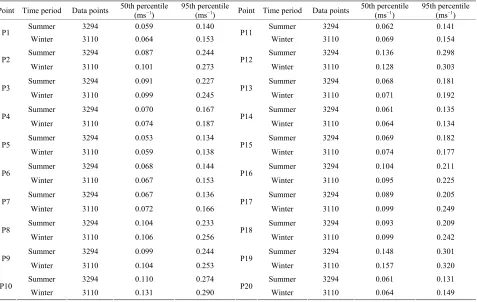
Table 3. Percentile analysis for the reference points (P1, P2, … P20) in the Black Sea for summer and winter time, respec-tively the second quartile and the 95th percentile.

Point Time period Data points 50th percentile _(ms−1₎ 95th percentile _(ms−1₎ Point Time period Data points 50th percentile _(ms−1₎ 95th percentile _(ms−1₎

Summer 3294 0.059 0.140 Summer 3294 0.062 0.141

P1

Winter 3110 0.064 0.153 P11 Winter 3110 0.069 0.154

Summer 3294 0.087 0.244 Summer 3294 0.136 0.298

P2

Winter 3110 0.101 0.273 P12 Winter 3110 0.128 0.303

Summer 3294 0.091 0.227 Summer 3294 0.068 0.181

P3

Winter 3110 0.099 0.245 P13 Winter 3110 0.071 0.192

Summer 3294 0.070 0.167 Summer 3294 0.061 0.135

P4

Winter 3110 0.074 0.187 P14 Winter 3110 0.064 0.134

Summer 3294 0.053 0.134 Summer 3294 0.069 0.182

P5

Winter 3110 0.059 0.138 P15 Winter 3110 0.074 0.177

Summer 3294 0.068 0.144 Summer 3294 0.104 0.211

P6

Winter 3110 0.067 0.153 P16 Winter 3110 0.095 0.225

Summer 3294 0.067 0.136 Summer 3294 0.089 0.205

P7

Winter 3110 0.072 0.166 P17 Winter 3110 0.099 0.249

Summer 3294 0.104 0.233 Summer 3294 0.093 0.209

P8

Winter 3110 0.106 0.256 P18 Winter 3110 0.099 0.242

Summer 3294 0.099 0.244 Summer 3294 0.148 0.301

P9

Winter 3110 0.104 0.253 P19 Winter 3110 0.157 0.320

Summer 3294 0.110 0.274 Summer 3294 0.061 0.131

P10

In statistical analysis, the standard deviation measures the data dispersion from the mean value as in Equation (1):





,

Std E_ X _ (1)

with E X

 

is the expectation operator. X represents a discrete ran-dom variable with the probability mass function p(x). Then the expected value will be:

 

 

E X 



In probability theory and statistics, skewness is a measure of the symmetry distribution in a certain data set. The skewness value can be positive, negative or unde-fined. The skewness of a variable X is defined as the

third standardized moment:

3 3

Skew  ,



 (3)

where ₃ is the third moment above the mean and the

kth moment about the mean is defined as:

 



k E X E X

  _ 



Kurtosis represents the relative concentration of the data in the centre versus in the tails of a frequency dis-tribution when is compared with the normal disdis-tribution (which has a kurtosis value of 3). This is equal to the fourth moment around the mean divided by the square of the variance (or the fourth power of the standard devia-tion) of the distribution minus 3.

4 4 3.

Kurt 



  (5)

Moreover, analyses regarding the 50th and 95th per-centiles were performed for all the points, grouped by summer time and winter time.

Percentiles are generally used in order to characterize a frequency distribution. In special the 50th and the 95th percentiles are often considered to identify the median values and the maximum data distributions being unaf-fected by outward values which are distant from the rest of the data. Percentiles (pi) are computed as follows:

0.5 100 , i i p n 

 (6)

where i represents the position inside the dataset that

marks the percentile to be calculated and n is the total number of the values in the distribution.

A first conclusion that can be drawn from Table 1 is that the average current velocity values in the Black Sea are in general small. There are usually small variations between summer and winter periods. The most stable points regarding velocity variations appear to be P1, P2,

P3, P4, P5 and P6. As expected, the points P1-P12 have higher current velocities than the rest, due to their coor-dinates located on the Rim current. The points P13, P14 and P15, located inside the curve described by the Rim current, have smaller velocities than the ones situated on the Rim or on the two anticyclonic eddies. The smallest velocity values are the ones recorded for the point P20, situated in the northwestern shelf zone, an area with mostly calm waters where no significant circulation fea-ture was observed.

3. Directional Distributions of the Current

Velocity

The rose type graphics are used to give a more compre-hensive picture of how current speeds and directions are distributed in a particular point. Using a polar coordinate system for gridding the frequency of the currents over the time period is plotted by current direction, with color bands showing current velocity ranges. The direction of the longest spoke shows the current direction with the greatest frequency. Each concentric circle represents a different frequency, starting from zero at the center with increasing frequencies at the outer circles. In Figures 3

and 4 rose graphics were drawn for the 20 reference points. Figure 3 presents rose graphics for the winter time, where winter is considered the time frame from October to March, while Figure 4 presents the rose graphics for the summer time (April to September).

By comparing Figure 3 and Figure4, it can be observed that there are significant changes between winter and summer time in current orientation, however these changes do not apply to all the points. P1, P5, P6, P11 and P13 present mostly the same structures for both time frames.

4. Comparisons against

in Situ

Data

For the Black Sea some current measurements were available for the time period 2002-2009 and they were compared against the corresponding satellite data pro-vided by Aviso. The measurements were taken at the Gloria drilling platform located on the western side of the Black Sea, near the Romanian coasts at 44˚31'N, 29˚34'E, every six hours. The data were then computed to a daily average, to fit the satellite data profile. The comparison between the satellite data and the measurements at the Gloria drilling platform in the Black Sea shows that the

in situ measured current velocity values are usually

higher than the satellite data with a bias of 0.077 ms−1_. Table 4 presents some statistical parameters as mean values, bias, RMS error, SI (scatter index) and r (correla-tion coefficient).

With Xi representing the measured values at the Gloria

drilling platform, Yi the corresponding satellite data

Figure 3. Current velocity roses for the reference points, winter time.

Figure 4. Current velocity roses for the reference points, summer time.

Table 4. Comparison between in situ measurements at the Gloria drilling platform and satellite data for the period 2002-2009.

Point Xmed (ms−1) Ymed (ms−1) Bias (ms−1) RMSE SI R

G 0.195 0.077 0.117 0.147 0.75 −0.025

statistical evaluated are defined by the following rela- tionships:

1

med ,

n i i

X

X X

n















1 RMSE , n i i i X Y n  





RMSE SI ,

X

 _ (10)









 



r . (11)

n i i i n n i i i i

X X Y Y

X X Y Y

       _{ }     







5. Discussions

According to satellite data the maximum current velocity is of 0.626 ms−1 _{and it belongs to P17, the point located}

at the edge of the Batumi eddy, closely followed by P19 with 0.588 ms−1 _{situated at the edge of the Sevastopol}

eddy, and P12 with 0.558 ms−1_{, situated on the Rim}

cur-rent. Except for the points P4 and P6, the current veloci-ties recorded on the Rim current are higher than the ones recorded inside. The minimum values are close to zero for all the points, while the mean values vary from 0.068 ms−1 _{for P14 to 0.160 ms}−1 _{for P19. The median values}

ranges from 0.056 ms−1 _{for P5 to 0.151 ms}−1 _{for P19.}

Higher values for the standard deviation suggest that the data is spread out compared to the mean values. A zero value for the skewness suggests that the values are rela-tively evenly distributed on both sides of the mean value while a positive skew indicates that the tail on the right side of the probability density function is longer than the left side and the bulk of values lie to the left of the mean, this being the case here where the skewness values range from 0.742 (P6) to 0.699 (P17). Kurtosis represents the relative concentration of the data in the center versus the tails of the frequency distribution when is compared to the normal distribution that has a kurtosis value of 3. In the present work the values of the kurtosis vary from 3.420 to 10.306.

For the winter time the point P1 is oriented towards south-west, feature that is preserved for the summer time, with a small peak added oriented towards north-east. Point P2 in the winter time shows also a south-west clear orientation, while for the summer this decreases, a peak oriented north-west being also added. Regarding P3, strong differences between winter and summer time can be observed. While in the winter is showing a strong south-east orientation, for the summer time this changes to north-west. P4 is showing a small north-east orienta-tion for the winter time, while for summer is difficult to

shelf area. While in the winter two dominant directions are present: north and south, for the summer there is a general orientation south.

5. Conclusions

As expected, most of the points located on the Rim cyc- lonic current and on the nearshore anticyclonic eddies have higher velocities than the ones located in the central gyres or northwestern shelf area. Also, they are described by a higher instability regarding current speed and direc- tion on the seasonal changes.

Higher value for kurtosis as the ones registered at points P5 (10.307), P17 (8.979), P13 (6.570) and P11 (6.219) means that in these cases there is a strong possi- bility that higher velocities than usual will appear.

A similar study with the emphasis on the anticyclonic and cyclonic eddies, was treated in [18]. The implemen- tation of a global circulation modeling system for the Black Sea basin was presented by Toderascu and Rusu in [19]. Also, the subject of modeling of wave-current in- teractions at the Danube mouths was treated by Rusu in [20]. Another work that needs to be mentioned here is the work of Rusu and Macuta regarding the numerical mod- eling of long shore currents in marine environment [21], as well as the work of L. Rusu regarding the application of numerical models to evaluate oil spills propagation in the coastal environment of the Black Sea [22].

6. Acknowledgements

The work of the first author has been made in the scope of the project EFICIENT (Management System for the Fellowships Granted to the Ph.D. Students) supported by the Project SOP HRD-EFICIENT 61445/2009. The al- timeter products were produced by Ssalto/Duacs and distributed by Aviso with support from Cnes.

This work was also supported by a grant of the Roma- nian Ministry of National Education, CNCS—UEFISCDI PN-II-ID-PCE-2012-4-0089 (project DAMWAVE).

REFERENCES

[1] D. M. Filippov, “The Cold Intermediate Layer in the Black Sea,” Oceanology, Vol. 5, No. 1, 1965, pp. 47-52. [2] D. Tolmazin, “Changing Coastal Oceanography of the

Black Sea in Northwestern Shelf,” Progress in Oceanog- raphy, Vol. 15. No. 4, 1985, pp. 217-276.

doi:10.1016/0079-6611(85)90038-2

[3] I. M. Ovchinnikov and Yu. I. Popov, “Evolution of the Cold Intermediate Layer in the Black Sea,” Oceanology,

Vol. 27, No. 3, 1987, pp. 555-560.

[4] C. E. Enriquez, “Mesoscale Circulation in the Black Sea: A Study Combining Numerical Modelling and Observa-tions,” Ph.D. Thesis, University of Plymouth, Devon, 2005, 257p.

[5] L. Mee and O. Maiboroda, “Black Sea Study Pack: A Resource for Teachers,” Black Sea Ecosystem Recovery Project, Vienna, 2006, 87p.

[6] N. M. Knipovich, “The Hydrological Investigations in the Black Sea Area,” Trudy Azova-Chernomorskoy Nauch-nopromyslovoy Ekspeditsii, Vol. 10, No. 10, 1932, 274p.

(in Russian)

[7] Filipov, “Circulation and Structure of the Waters in the Black Sea,” Nauka, Moscow, 1968, 136p.

[8] S. G. Boguslavskiy and A. S. Sarkisyan, T. Z. Dzhioyev and L. A. Koveshnikov, “Analysis of Black Sea Current Calculations,” Izvestiya Atmospheric and Oceanic Phys-ics, No. 12, 1976, pp. 205-207.

[9] A. S. Blatov, N. P. Bulgakov, V. A. Ivanov, A. N. Ko-sarev and V. S. Tuljulkin, “Variability of the Black Sea Hydrophysical Fields,” Gydrometeoizdat, Leningrad, 1984, 240p.

[10] E. V. Stanev, D. Truhchev and V. Roussenov, “Black Sea Circulation and Its Numerical Modeling,” St. Kliment Ohridski University Press, Sofia, 1984, 222p.

[11] E. V. Stanev, “On the Mechanisms of the Black Sea Cir-culation,” Earth Science Reviews, Vol. 28, No. 4, 1990,

pp. 285-319. doi:10.1016/0012-8252(90)90052-W [12] V. N. Eremeev, A. V. Ivanov and V. S. Tuljulkin,

“Cli-matic Interannual Variability of Geostrophic Circulation in the Black Sea,” Ukrainian Academy of Sciences, Kyiv, 1991, 53p.

[13] T. Oguz, V. S. Latun, M. A. Latif, V. V. Vladimirov, H. I. Sur, A. A. Markov, E. Ozsoy, B. B. Kotovchchikov, V. V. Eremeev and U. Unluata, “Circulation in the Surface and Intermediate layers of the Black Sea,” Deep Sea research I, Vol. 40, No. 8, 1993, pp. 1597-1612.

doi:10.1016/0967-0637(93)90018-X

[14] T. Oguz, M. A. Latif, H. I. Sur, E. Ozsoy and U. Unluata, “The Black Sea Circulation: Its Variability as Inferred from Hydrographic and Satellite Observations,” Journal of Geophysical Research: Oceans, Vol. 97, No. C8, 1992,

pp. 12569-12584. doi:10.1029/92JC00812

[15] J. Staneva, D. Dietrich, E. Stanev and M. Bowman, “Rim Current and Coastal Eddy Mechanisms in an Eddy-Re- solving Black Sea General Circulation Model,” Journal of Marine Systems, Vol. 31, No. 1-3, 2001, pp. 137-157. doi:10.1016/S0924-7963(01)00050-1

[16] G. Korotaev, T. Oguz, A. Nikiforov and C. Koblinsky, “Seasonal, Interannual, and Mesoscale Variability of the Black Sea Upper Layer Circulation Derived from Al- timeter Data,” Journal of Geophysical Research, Vol. 108,

No. C4, 2003, p. 3122. doi:10.1029/2002JC001508 [17] http://www.aviso.oceanobs.com/en/

[18] R. Toderascu and L. Rusu, “Study on the Currents Vari-ability and Patterns in the Black Sea,” 12th International Multidisciplinary Scientific GeoConference SGEM 2012,

17-23 June 2012, pp. 825-832.

http://sgem.org/sgemlib/spip.php?article2190

http://sgem.org/sgemlib/spip.php?article2179&lang=en [20] E. Rusu, “Modeling of Wave-Current Interactions at the

Danube Mouths,” Journal of Marine Science and Tech-nology, Vol. 15, No. 2, 2010, pp 143-159.

doi:10.1007/s00773-009-0078-x

[21] E. Rusu and S. Macuta, “Numerical Modelling of Long-shore Currents in Marine Environment,” Environmental

Engineering and Management Journal, Vol. 8, No. 1,

2009, pp. 147-151.

[22] L. Rusu, “Application of Numerical Models to Evaluate Oil Spills Propagation in the Coastal Environment of the Black Sea,” Journal of Environmental Engineering and Landscape Management, Vol. 18, No. 4, 2010, pp. 288-