Munich Personal RePEc Archive
How a fast lane may replace a congestion
toll
Fosgerau, Mogens
Technical University of Denmark
2011
How a fast lane may replace a congestion toll
Mogens Fosgerau
yMarch 10, 2011
Abstract
This paper considers a congested bottleneck. A fast lane reserves a more than proportional share of capacity to a designated group of travellers. Travellers are otherwise identical and other travellers can use the reserved capacity when it would otherwise be idle. The paper shows that such a fast lane is always Pareto improving under Nash equilibrium in arrival times at the bottleneck and inelastic demand. It can replicate the arrival schedule and queueing outcomes of a toll that optimally charges a constant toll during part of the demand peak. Within some bounds, the fast lane scheme is still welfare improving when demand is elastic.
Keywords: congestion; tolling; bottleneck; scheduling; fast lane
1
Introduction
This paper considers a fast lane scheme as a means to regulate congestion in a regularly occurring demand peak. The fast lane scheme plays explicitly on the dynamics of congestion, which makes the Vickrey (1969) bottleneck model an appropriate framework. The elements of the basic bottleneck model are a description of the queueing technology in the bottleneck, a continuum of
Technical University of Denmark ([email protected]), Centre for Transport Stud-ies, Sweden and Ecole Normale Supérieure de Cachan, France.
yThis research is supported by the Danish Social Science Research Council. In addition,
identical travellers with scheduling preferences who have to pass the bottle-neck, and the concept of Nash equilibrium in arrival times at the bottleneck. The fast lane scheme allocates the bottleneck capacity to di¤erent classes of travellers. The scheme is the following.
A set of travellers is assigned to a priority group. Not all travellers can be given priority. A more than proportional share of capacity is reserved for the priority group. When the reserved capacity is not used, it is available for the nonprioritized travellers.
This is similar to, e.g., the check-in in airports with separate queues and servers for economy and business class passengers. Whenever the business class server is idle, it may serve passengers from the economy class queue. Another example is the HOV or HOT lanes as found on US motorways. Yet another example is the ‡ows at di¤erent motorway on-ramps that could be given di¤erent priority (Shen and Zhang (2010) consider such a scheme). Even though such a scheme it is called a fast lane scheme in this paper, the de…nition encompasses many other policies that do not involve the allocation of road lanes for di¤erent classes of vehicles; it is more general than allocation of lanes.
The paper compares the fast lane scheme to tolling. Like Arnott et al.
(1990), this paper considers a coarse toll, which is a constant toll that applies only during part of the peak.1 Arnott et al. (1990) found that Nash
equi-librium under a coarse toll comprises a point mass in the arrival schedule at the time when the toll is lifted. This is an undesirable feature of their model as such point masses are physically implausible. The problem is avoided in this paper by a reformulation of the queueing technology. In this paper, the congestion technology is such that travellers who choose not to pay the toll can queue at the same time as travellers who are paying the toll pass the bottleneck. This is also true of the examples of fast lanes given above. In this case, a point mass in the arrival schedule does not arise. The analy-sis below uses the reformulated queueing technology and repeats the Arnott et al. (1990) analysis of a coarse toll under this assumption.
The …rst main result of this paper is that the fast lane scheme is always Pareto improving when demand is not price sensitive. There are no restric-tions on how large the group of prioritized travellers should be as long as it is …xed exogenously. Prioritized travellers experience a strict utility gain while the properties of Nash equilibrium imply that nonprioritized travellers do not lose. It is signi…cant that this occurs even when travellers are homogenous and there are no toll payments. This robustness is very desirable since it
1Arnott et al.(1990) applied also a base toll level. This paper considers the coarse toll
means that a regulator needs little information to implement the scheme and be certain to achieve a welfare improvement. In fact, the regulator can mon-itor tra¢c in real time and assign capacity accordingly. This is consistent with the way the fast lane scheme is formulated in the model. With price sensitive demand, the fast lane scheme is still welfare improving if the price elasticity of demand is not too high and the share of prioritized travellers is not too large.
The second main result of this paper is that the fast lane scheme can reproduce the equilibrium arrival pattern of the optimal coarse toll when demand is not price sensitive.2 In fact, the scheme can reproduce the
equi-librium arrival pattern of any coarse toll, provided that the tolling interval is the same as the arrival interval that a prioritized group would endogenously select. This is signi…cant since the fast lane scheme has a number of advan-tages over tolling. First, the fast lane scheme is always welfare improving and can be adjusted in real time. In order to set the right coarse toll it is necessary to know exactly when to start and when to end the tolling inter-val. Mistakes will reduce the welfare gain from tolling and can even lead to a welfare loss. Second, it is plausible that system costs can be a lot lower for a fast lane scheme than for a toll as the fast lane does not involve any payment. Finally, as there is no payment, a fast lane scheme may be more acceptable to travellers than tolling. Within the simple theoretical model presented here, prioritized travellers would be strictly better o¤ under the fast lane scheme than under no policy, while the remaining travellers would be indi¤erent. In contrast, all travellers would be indi¤erent between tolling and no policy as toll revenues are not returned to travellers. This property of fast lanes may explain why fast lanes have been introduced while there is generally a reluctance to introduce tolls.
A notable feature of the present paper is the formulation of scheduling utility which generalizes those employed by Vickrey (1969, 1973), Arnott et al. (1990, 1993), and many others. Here, scheduling utility is taken to be a strictly concave function of times at which the trip starts and ends. Travellers prefer to depart later and to arrive earlier. For any …xed travel time there is a unique preferred departure time. These assumptions are su¢cient for the results of this paper. The paper establishes that the socially optimal fast lane scheme achieves more than half the welfare gain of the
2Using scheduling preferences,Knockaert et al.(2010) show that the coarse
socially optimal continuously time varying toll. This generalizes the parallel result by Arnott et al. (1990) for the coarse toll under their …rst-in-…rst-out congestion technology to the present formulation of scheduling utility combined with parallel queueing.
Section2presents the model setup. Section3considers the Nash equilib-rium under no policy. Section 4 analyses the coarse toll. Section 5 analyses the fast lane scheme. Section6extends to the case of price sensitive demand. Section 7concludes.
2
The bottleneck model of congestion
Travellers depart from some origin to arrive at the back of the queue at a bottleneck after a travel time of d0 minutes. The queue has no physical
extension. Travellers have to pass through the bottleneck to reach their destination. Travel time after exiting the bottleneck is d1 minutes. The
bottleneck serves the queue at the capacity rate of travellers per minute. Travellers and capacity may be split such that only a time-varying part of capacity i(s)is available to travellers of classi:There is a separate queue for
each class of travellers such that it is possible for some classes to queue while others pass the bottleneck. The class i queue at the bottleneck has length
Qi(a) 0 at time a: Travellers arrive at the bottleneck at the rate i(a)
during some interval[a0; a1]with the total number of classitravellers having
arrived at time a beingRi(a) =
Ra
a0 i(s)ds:The queue evolves according to
Qi(a) =Ri(a)
Z a
a0
i(s) 1fQi(s)>0g+ min ( i(s); i(s)) 1fQi(s)=0g ds:
A traveller who arrives at the bottleneck at time a; exits the bottleneck at timeti(a)given implicitly byQi(a) =
Rti(a)
a i(s)ds:When there is only one
class such that capacity is …xed at and if Q(s) >0 for all s 2int[a0; a];
then t(a) =R(a)= +a0:
The preferences of travellers are expressed by a utility function, which is a function of the departure time from the origin, the arrival time at the destina-tion and a toll associated with the trip. This is writtenu(a d0; t+d1) ;
whereuis called the scheduling utility, ais the arrival time at the bottleneck,
d0 is the travel time from the origin to the back of the queue at the
bottle-neck, t is the time of exit from the bottleneck, d1 is the travel time from the
the bottleneck to maximize utility. The function v(a) =u(a; a) is assumed to attain maximum, which says there is an optimal time at which travellers would prefer to go if travel was instantaneous. The distances d0 and d1 are
normalized to zero at no loss of generality. Travellers are identical except for an observable characteristic which does not a¤ect utility and which can-not be in‡uenced by travellers. The characteristic is observable by the road operator and can be used to form groups of any size.
The model is closed by assuming Nash equilibrium, which holds that no traveller is able to strictly increase utility by changing arrival time at the bottleneck, taking the arrival schedule of all other travellers as given. With identical travellers this implies that all travellers of class i achieve the same utility, denoted by i:The welfare function is the total consumer surplus plus
total toll revenues plus a constant to be explained below. Denoting demand for class i by ni and the total toll payment by T;the welfare function is
W =P
i
Z 0
i
ni(c)dc+T
The constant in the welfare function occurs because the upper integral limit is …xed at 0in order to accommodate situations with a price elasticity of demand of zero.
3
No policy Nash equilibrium for one class
The analysis of no policy Nash equilibrium is carried out allowing for variable capacity ( )as it will allow results to be reused below. In Nash equilibrium, travellers will arrive during an interval [a0; a1] determined by the equations
N = Ra1
a0 (s)ds and v(a0) =v(a1): This means that there is no queue at
these endpoints, Q(a0) = Q(a1) = 0: There is a strictly positive queue at
any time in the interior of this interval. The arguments for this are easy and will not be repeated here (de Palma and Fosgerau, 2009). This implies that the expression for the queue length simpli…es to
Q(a) = R(a)
Z a
a0
(s)ds
and so the implicit expression for the time of exit becomes
R(a) =
Z t(a)
a0
Therefore, by di¤erentiation, (a) = (t(a))t0(a): Di¤erentiation of the
identity u(a; t(a)) = given by the equilibrium condition leads to
0 = u1(a; t(a)) +u2(a; t(a))t0(a)
= u1(a; t(a)) +u2(a; t(a))
(a)
(t(a));
such that the equilibrium arrival rate may be expressed as
(a)
(t(a)) =
u1(a; t(a))
u2(a; t(a))
:
The welfare function has the value W = N =v(a0)N:
4
Coarse tolling
This section considers a coarse toll, de…ned to be a toll that is zero except in an interval during the peak where it takes a …xed value :Denote this interval by[b0; b1]:The toll applies at the front of the queue, when the traveller passes
the bottleneck. The toll splits travellers into two classes according as they choose to travel at a time when the toll applies or not. There are separate queues for these two classes.3
The coarse toll should be small enough and the tolling interval be brief enough that it does not lead to unused capacity. Let therefore the toll be such that v(b0) :Otherwise, a traveller arriving at the bottleneck at
or just after time b0 will be worse of than in Nash equilibrium, even when
there is no queue at time b0: Hence nobody will travel at time b0 and there
will be unused capacity. Similarly, the toll must have u(b1; b1) :By
concavity of scheduling utility, these conditions imply that v(a)
for all a 2 [b0; b1]: Together the conditions ensure that there is not unused
capacity under the toll. Another consequence is that the arrival interval
[a0; a1] is unchanged relative to Nash equilibrium. This in turn implies that
the equilibrium utility is still :
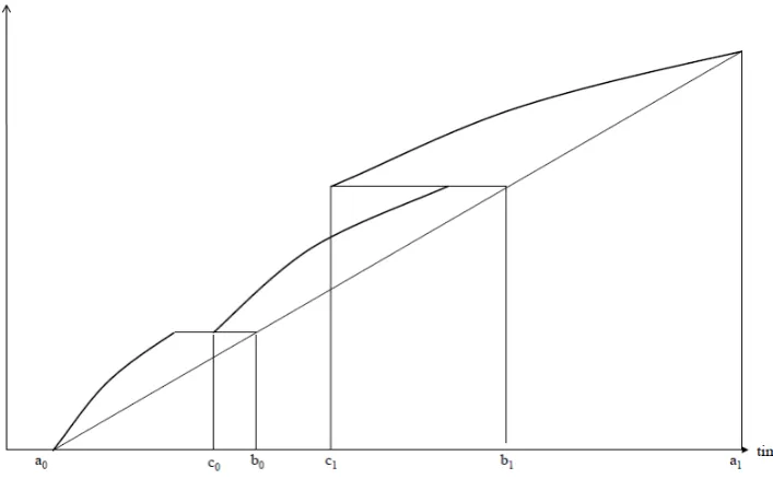
The Nash equilibrium that results under a coarse toll that does not lead to unused capacity is illustrated in …gure ??. Arrivals start at time a0 and
follow the no policy Nash equilibrium schedule until just before the …rst arrival time where the traveller must pay the toll: Nash equilibrium requires that utility is also for the …rst traveller to pay the toll. Therefore there
3The Stockholm congestion charge varies in steps over the peak. Anecdotes from
Figure 1: Arrival schedule under coarse toll
must be an interval with no new arrivals at the bottleneck. Arrivals resume at the time c0 when =u(c0; b0) : Then arrivals continue until the last
time when the traveller must pay the toll. Later travellers who will not pay the toll begin queueing in their own queue at time c1 to follow the arrival
schedule of the no policy equilibrium.
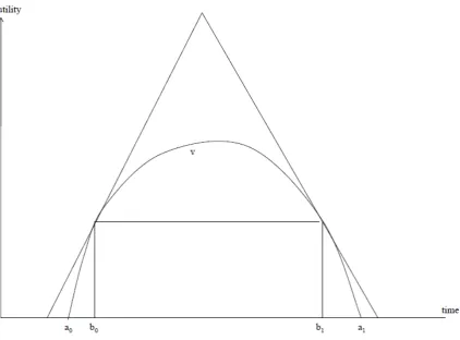
The optimal coarse tolling interval starts early enough and ends late enough that
=u(b0; b0) =u(b1; b1) : (1)
This is illustrated in …gure 2.
The welfare maximizing toll …nds such that total scheduling utility is maximal. This is equivalent to maximizing toll revenue since the utility of every traveller is in equilibrium. The toll revenue is (b1 b0):
Maxi-mizing toll revenue requires the …rst order condition
(b1 b0) +
@(b1 b0)
@ = 0:
The endpoints of the tolling interval are such that
1 = @v(b0)
@b0
@b0
@ =
@v(b1)
@b1
@b1
Figure 2: Arrival schedule under coarse toll with optimal tolling interval given size of toll
Hence the optimal toll satis…es
= 1(b1 b0)
@v(b1) @b1
1
@v(b0) @b0
>0: (2)
The following statement uses the theorem-proof format as the proof is fairly long. LetWebe the welfare measure for the no policy Nash equilibrium.
Index similarly the optimal coarse toll equilibrium with c and the social optimum with a time varying toll by so:The theorem states that the coarse toll captures at least half the welfare gain of the socially optimal time varying toll.
Theorem 1
Wso We
2 Wc We:
Proof. The function v is shown on …gure 3. Time is on the horizontal axis and utility in monetary terms is on the vertical axis. All travellers receive utility v(a0) = v(a1) in no policy Nash equilibrium. Under the socially
optimal time varying toll travellers arrive at the bottleneck during [a0; a1] at
the rate and there is no queueing. HenceWso =
Ra1
corresponds to the area under v and over the horizontal line intersecting v
at a0 and a1:
Introducing a bit of shorthand notation, the optimal coarse toll is given in (2) by
= b11 b0
v0 1 1 v0 0 :
Consider the triangle, shown in …gure 3, which has the horizontal line as baseline and edges that are tangent to v at (b0; v(b0)) and (b1; v(b1)): This
triangle is strictly greater than Wso We since v is strictly concave. The
baseline of the triangle is hb0 v0
0; b1 v01 i
: Parametrizing the edges of the triangle, the edges cross at the point xon the baseline given by the equation
v0
0 x b0+v0
0 = v
0
1 x b1+ v0
1 with solution x =
v0
1b1 v00b0
v0
1 v00 : The height
of the triangle is then
v00 x b0+
v0
0
= v00 v
0
1b1 v00b0
v0
1 v00
b0 +
v0
0
= v00 v
0
1b1 v00b0 b0(v10 v00)
v0
1 v00
+
= v
0
0v10
v0
1 v00
(b1 b0) + = 2 :
It follows that the area of the triangle is b1 b0 v0
1 + v00 = 2 (b1 b0);
such that Wso We 2 (b1 b0): The welfare gain from the coarse toll is
equal to the toll revenue Wc We= (b1 b0):
The statement of the Theorem holds with equality, i.e. Wso We =
2 (Wc We);when scheduling preferences are piecewise linearu(a; t) =
(t a) min (t;0)+ max (t;0):Hence the bound in the Theorem cannot
be improved in general.
5
Fast laning
This section considers a fast lane scheme. The suggested scheme is the follow-ing. Based on the observable characteristic of travellers, an operator assigns travellers to two classes with N1 and N2 travellers. The preferences of
reserved for class 1 travellers where
0< N1
N <
1
1: (3)
Class 2 travellers are allowed to use all of capacity when there are no class 1 travellers queueing. Otherwise they can only use the remaining capacity
1:
This section establishes the two main results of this paper. The …rst result is that such a scheme is always Pareto improving. This is in contrast to a coarse toll, which may reduce welfare by causing idle capacity during
[a0; a1] if the toll is too high or lasts for too long. The second result is that
the scheme can achieve exactly the same travel time and queueing outcomes as a coarse toll satisfying the partial optimality conditions that the tolling interval equalizes the utility of the travellers at the endpoints (1).
To establish that a fast lane scheme is always Pareto improving, consider …rst the behavior of class 1. Since N1= 1 < N= , they are able to pass the
bottleneck in a shorter interval than [a0; a1]:They form a Nash equilibrium
during an interval [b0; b1] with a0 < b0; b1 b0 =N1= 1; b1 < a1 and v(b0) =
v(b1): These travellers therefore achieve a strict utility gain relative to the
basic Nash equilibrium, v(v1)> .
The remaining class 2 travellers, form a Nash equilibrium using the re-maining capacity. The rere-maining capacity is 1 during[b0; b1]and
oth-erwise. All class 2 travellers are able to pass the bottleneck during [a0; a1]:
They therefore form Nash equilibrium with variable capacity as described in section3and the resulting equilibrium utility is :This establishes that any fast lane scheme satisfying (3) will be Pareto improving.
The next point is to establish that the fast lane scheme can achieve ex-actly the same travel time and queueing outcomes as a coarse toll satisfying the partial optimality conditions. So consider a toll during [b0; b1]
satis-fying (1). This is the kind of situation depicted in …gure 2. Note that toll paying travellers occupy all the bottleneck capacity during [b0; b1] and that
these travellers do not queue at timesb0andb1:Hence their behavior is
repro-duced under a scheme that assigns (b1 b0)travellers into class 1 and gives
them all the capacity 1 = , while the remaining travellers are assigned to
6
Fast lane with price sensitive demand
The no policy equilibrium scheduling utility depends only on the time it takes all travellers to pass the bottleneck N:Introduce a cost functionc N =
equal to the negative of the equilibrium scheduling utility. By the assump-tions made, c is strictly increasing and strictly convex. Assume that de-mand is price sensitive with dede-mand given as a decreasing function n(c)
of scheduling cost. Combine the functions n and c into a new function as
f N =n c N :Then N =f N in no policy Nash equilibrium.
Consider now a fast lane scheme that divides the population of potential travellers into two classes with proportions and 1 : The allocation of travellers to classes is based on the observable characteristic which cannot be in‡uenced by travellers. The division of the population of potential travellers into classes gives rise to two demand curves n( )and (1 )n( ):
Let N1; N2 be the equilibrium number of travellers in the two classes,
where group 1 is the priority class and capacity is assigned such that 0 <
N1
N1+N2 <
1 1: As shown, the equilibrium cost for class 1 travellers is
c(N1= 1); such that the equilibrium number of class 1 travellers is N1 =
f N1
1 :Similarly, the equilibrium cost for class 2 travellers isc(N= )such
that equilibrium requires that N2 = (1 )f N1+N2 :
It has already been shown that such a fast lane scheme is welfare im-proving when demand is not price sensitive. It follows by continuity that the scheme is also welfare improving when the price elasticity of demand is su¢ciently small. The remainder of this section shows that the scheme is welfare improving when the share is su¢ciently small.
The no policy Nash equilibrium results when 1 = : The following
derivatives will be useful. They show that increasing while holding 1 constant increases the number of class 1 travellers and decreases the number of class 2 travellers.
@N1
@ = f
N1
1
+
1
f0 N1
1
@N1
@ =
f N1 1
1
1f
0 N1 1
>0
@N2
@ = f
N1+N2
+ 1 f0 N1+N2 @N1
@ +
@N2
@
=
f N1+N2 1 f0 N1+N2 @N1
@
1 1 f0 N1+N2
The expression for @N2
@ is composed of two negative terms. The …rst is the
direct e¤ect on N2 of changing ; the second term is the e¤ect through the
cost. The second term is negative indicating that the cost is increasing. This indicates that unprioritized travellers lose as increases such that larger does not lead to a Pareto improvement. The following derivation shows that the total number of travellers strictly decreases as increases.
@N1
@ +
@N2
@ =
@N2
@ +f
N1+N2
1 f0 N1+N2
=
@N1
@ +f
N1+N2
1 1 f0 N1+N2
<0 (4)
The welfare function with variable demand is de…ned as the consumer surplus
W =
Z 1
c N1 1
n(c)dc+ (1 )
Z 1
c(N1+N2)
n(c)dc:
Di¤erentiation with respect to yields
@W
@ =
Z c(N1+N2 )
c N1 1
n(c)dc N1
1
c0 N1
1
@N1
@
N2
c0 N1+N2 @N1
@ +
@N2
@ :
Evaluating at = 0 yields
@W
@ =
N2
c0 N1+N2 @N1
@ +
@N2
@ :
This is strictly positive by (4). Continuity implies that there is always some
>0 such that the fast lane scheme is welfare improving. Further simpli…-cations do not seem to be available.
7
Conclusion
It is straightforward but tedious to generalize the results of this paper to tolls with more steps and fast laning schemes with more user classes.4 The
4Laih(1994) showed that it is straightforward to extend the coarse toll to a multistep
toll. It is similarly straightforward to extend a fast lane scheme in this way. Laih (1994)
general conclusion remains that fast laning can achieve the same bene…ts as step tolls when demand is not price sensitive. It is also straightforward to see that a sequence of step tolls, and hence a sequence of fast laning schemes, can be constructed that approach the optimal time varying toll. In the limit, the step toll would become the optimal continuously varying toll while the fast lane scheme would become equivalent to allocating a speci…c time slot to every traveler.
A potentially useful feature of the fast lane scheme is its robustness. As long as demand is not too elastic, or as long as the share of prioritized travellers is no too large, then any fast lane scheme satisfying (3) is welfare improving. If demand is not price sensitive, then any such fast lane scheme is Pareto improving. An interesting direction for further inquiry is how this robustness can be utilized. Is it the case that the fast lane scheme retains its favorable properties when some element of stochasticity is introduced into the model?
References
Arnott, R. A., de Palma, A. and Lindsey, R. (1990) Economics of a bottleneck
Journal of Urban Economics27(1), 111–130.
Arnott, R. A., de Palma, A. and Lindsey, R. (1993) A structural model of peak-period congestion: A tra¢c bottleneck with elastic demandAmerican Economic Review 83(1), 161–179.
de Palma, A. and Fosgerau, M. (2009) Random queues and risk averse users
Working Paper .
Knockaert, J., Verhoef, E. T. and Rouwendal, J. (2010) Bottleneck Conges-tion: Di¤erentiating the Coarse Charge Working Paper .
Laih, C.-H. (1994) Queueing at a bottleneck with single- and multi-step tolls
Transportation Research Part A28(3), 197–208.
Laih, C. H. (2004) E¤ects of the optimal step toll scheme on equilibrium commuter behaviour Applied Economics 36(1), 59–81.
Shen, W. and Zhang, H. M. (2010) Pareto-improving ramp metering strate-gies for reducing congestion in the morning commute Transportation Re-search Part A44(9), 676–696.
Vickrey, W. S. (1969) Congestion theory and transport investmentAmerican Economic Review 59(2), 251–261.