Study on A Standing Wave Thermoacoustic Refrigerator
Made of Readily Available Materials
Jinshah B S*, Ajith Krishnan R**, Sandeep V S***
*Department of Mechanical Engineering, Government Engineering College, Kozhikode, Kerala, India **Department of Mechanical Engineering, Government Engineering College, Kozhikode, Kerala, India ***Department of Mechanical Engineering, Government Engineering College, Kozhikode, Kerala, India
Abstract- Use of CFC-contained systems has caused severe environmental hazards that have researchers looking for alternatives. Studies have shown that thermoacoustic technology is suited a candidate for conventional vapour compression cooling system in particular for special uses. In this research, theoretical, numerical and experimental studies were completed to identify optimum operating conditions for the design, fabrication, and operation of a thermoacoustic refrigerator. The system uses no refrigerant or compressor, and the only mechanical moving part is the loudspeaker connected to a signal generator that produces the acoustics. Here air at 1 atm is used as the working gas. The system fabricated with this grant is made of PVC and brass with a sinusoidal section to reduce power loss and can operate up to a maximum of 4 bar. The system can be taken apart if different stack geometry or material is to be studied.
Index Terms- Standing wave thermoacoustic refrigerator, stack, resonator column, acoustics, stirling cycle
I. INTRODUCTION
hermoacoustics, as defined by Rott is a subject dealing generally with effects in acoustics in which heat conduction and entropy variations of a medium play a role. In this study the term thermo acoustics will be used in the limited sense of the generation of sound by heated surfaces and the process of heat transfer from one place to another by sound. In this section a brief review of the history of thermoacoustics is presented, along with a simple physical explanation of the effect, and some applications.
The development of thermoacoustic refrigeration is driven by the possibility that it may replace current refrigeration technology. Thermoacoustic refrigerators, which can be made with no moving parts, are mechanically simpler than traditional vapour compression refrigerators and do not require the use of harmful chemicals. Because of their simplicity, TARs should be much cheaper to produce and own than conventional technology. The parts are not inherently expensive, so even initial manufacturing costs should be low. Furthermore, mechanical simplicity leads to reliability as well as cheaper and less frequent maintenance. Until efficiency can be improved, operation costs may be higher; but with fewer moving parts, TARs require little to no maintenance and can be expected to have a lifetime much longer than ordinary refrigeration technology. Also, efficiency is likely to improve as thermoacoustic technology matures. Therefore, thermoacoustic refrigeration is likely to be more cost effective.
Besides reduced financial cost, environmental cost should be considered. Traditional vapour compression systems achieve their efficiencies through the use of specialized fluids that when released into the atmosphere (accidentally or otherwise) cause ozone depletion or otherwise harm the environment. Even most of the alternative fluids being developed cause harm in one way or another. For example, propane and butane won’t destroy the ozone, but are highly flammable and pose a threat if a leak should occur. On the other hand, TARs easily accommodate the use of inert fluids, such as helium that cause no harm to the environment or people in the event of a leak. Also, normal operating pressures for TARs are about the same as for vapour compression systems, so thermoacoustic refrigeration is just as safe in that respect. Furthermore, TARs can be driven by TAEs in which case the input power can come from any source of heat, including waste heat from other processes. Then the combination TAE/TAR device has no negative impact on the environment and, in fact, can utilize energy sources that are otherwise wasted. Overall, thermoacoustic refrigeration is much more benign than conventional refrigeration methods in terms of environmental and personal safety.
One drawback, however, is a lack of efficiency in current TARs when compared to vapor compression. Traditional refrigeration techniques have the benefit of generations of research and application whereas thermoacoustic refrigeration is a new technology, so it is no wonder that vapour compression refrigerators are currently more efficient; however, there is reason to believe that thermoacoustic refrigeration will overtake vapour compression in the long run. The major reason is that a TAR can be driven with proportional control, but vapour compression schemes are binary (on/off). Although standing-wave TARs are currently less efficient than comparable conventional refrigerators, some of the difference can be made up when less than full power is required, which is most often the case. A normal refrigerator must switch off and on to maintain a given temperature; so the compressor is working its hardest whenever it is on, and the temperature actually oscillates around the desired value. In contrast, a refrigerator capable of proportional control, such as a TAR, can tune its power output to match the requirements of the load; so if the load increases a small amount, the refrigerator can slightly increase its power for a short time rather than running full tilt. This is especially advantageous in
applications where thermal shocks can cause damage, such as cooling electronics. As indicated above, it is absolutely possible—if not probable—that with expanded research efforts, thermoacoustic technology will become more efficient than vapour compression.
Due to its advantages in mechanical simplicity and environmental and personal safety, thermoacoustic refrigeration is becoming more important in the research community and may soon reach a point in its development when it can replace vapour compression as the primary technology used in refrigeration applications.
II. HISTORY
[image:2.612.271.371.197.321.2]The generation of acoustic oscillations by heat have been observed and studied for over two centuries. Byron Higgins made the first observations and investigations of organ-pipe type oscillations, known as singing flames in 1777. At certain positions of a hydrogen flame inside a tube, open at both ends, acoustic oscillations were observed. Fig.(2.1) shows a configuration for producing Higgins oscillations. A survey of the phenomena related to Higgins oscillations was given by Putnam and Dennis.
Figure 2.1: One form of the singing-flame apparatus. For certain position of The flame inside the tube acoustic oscillations can be observed
[image:2.612.276.385.441.645.2]In 1859, Rijke discovered that strong oscillations occurred when a heated wire screen was placed in the lower half of an open-ended pipe, as shown in Fig.(2.2). It was noticed that the convective air current through the pipe was necessary for the phenomenon to occur. Oscillations were strongest when the heated screen was located at one-fourth of the length of the pipe from the bottom end. Feldman gave a review of the literature on the Rijke tube [.Probably the research by Sondhauss, performed in 1860, approximates best what we define today as thermoacoustic oscillations. Sondhauss studied experimentally heat-generated sound, observed for centuries by the glass-blowers when blowing a hot bulb at the end of a cold narrow tube.
Figure 2.2: Rijke tube. The rijke acoustic oscillations can be observed best with the heated wire screen at one-fourth of the pipe from the bottom end
1962 Carter, during an experimental investigation of the feasibility of the Sondhauss tube to generate electricity, found that the insertion of a bundle of small glass tubes inside the Sondhauss tubes improved their performance. In 1887, Lord Rayleigh gave a qualitative explanation, in his classic work on sound for the Sondhauss oscillations. If heat be given to the air at the moment of greatest condensation or taken from it at the moment of greatest rarefaction, the vibration is encouraged. So Rayleigh knew that thermoacoustics was due to the interplay of heat injection and density variations.
Figure 2.3: Soundhauss tube. When heat is supplied for example by means of a flame to the closed end, sound can be generated
Another form of Sondhauss oscillations, which occur in cryogenic storage vessels, are the so called .Taconis oscillations.. Taconis observed spontaneous oscillations when a hollow tube with the upper end closed was inserted in liquid helium. Taconis explanation of how the large temperature gradient along the tube caused the oscillations was essentially a restatement of the Rayleigh criterion. The Taconis oscillations have been studied experimentally by Yazaki et al. Although various aspects of what is now known as thermo acoustics have been of interest for centuries, the formal theoretical study of thermoacoustics started in 1949, when Kramers studied the Taconis oscillations. He generalized the Kirchhoff theory of the attenuation of sound waves at constant temperature to the case of attenuation in the presence of a temperature gradient. The results of Kramers theory were in disagreement with the experiment, because of some incorrect assumptions. In 1969, Rott continued the work of Kramers in a series of papers where a successful linear theory of thermoacoustics is given. Wheatley, Swift, and others have developed the connection between the acoustical part of thermo acoustics in a broader thermo dynamical perspective. Swift has reviewed much of this work. As can be understood from the above discussion, the history of heat-driven oscillations is rich and old. But the reverse thermodynamic process, of generating a temperature gradient by imposing acoustic oscillations, is a more recent phenomenon. Gifford and Longsworth demonstrated a heat-pumping process along the inner surface of a closed tube, where pressure pulses at low frequency were sustained . They called this cooling device a .Pulse tube, which is the precursor of the present orifice pulse-tube coolers. In 1975, cooling was also observed by Merkli and Thomann , at the velocity antinodes of a cylindrical cross-section acoustic tube in resonance. These two events formed the start of the work at Los Alamos National Laboratories (LANL) on thermoacoustic devices in the eighties, by Wheatley, Swift, and coworkers. The first acoustic heat pump (cooler), built at LANL, used a loudspeaker at one end of a closed tube to drive the acoustic resonance, and a stack of fiber glass plates positioned at the opposite end. The stack of plates was used to improve the thermoacoustic effect, as observed by Carter et al. With this arrangement, it was easy to produce a temperature difference over the stack, as a result of the heat transfer process from one end of the stack to the other. Since then, several experimental set-ups have been built.
III. BASIC PRINCIPLE OF THE THERMOACOUSTIC EFFECT
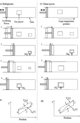
Acoustic waves consist not only of coupled pressure and displacement oscillations in a gas, but also of temperature oscillations as a response to the pressure variations. The interaction of these effects in gas close to a solid surface generates thermoacoustic oscillations. At the surface, heat can be extracted or supplied to the gas. The result of this interaction is that a sound wave is sustained in case of a large temperature gradient along the surface. While in the reverse case acoustic work is absorbed in order to transport heat, generating a temperature gradient. The mechanism of the thermoacoustic effect can best be visualized by considering a tube containing a gas, closed at one end and at the other an oscillating piston is moving forwards and backwards, compressing and expanding the gas in the tube, as shown in Fig.(3.1). In order to understand how the thermoacoustic cycle works, we follow a small volume of gas (parcel), as indicated by the small square in Fig(3.1), as it moves alongside the wall of the tube.
and heat transfer from the wall to the parcel takes place (4). At this moment, the parcel of gas is at the initial position, and the cycle starts again.
Figure 3.1: A typical gas parcel executing the four steps (1-4) of the cycle in a thermoacoustic refrigerator (left side)and prime mover (right side), assuming an inviscid gas and square wave acoustic motion and pressure. In each step, the dashed and solid squares are vertical triangles show the initial and final states of the parcel and piston, respectively. (b) gas temperature Tg(x), and wall temperature
Tw(x)versus position of the refrigerator. (d)Gas temperature Tg(x), and Wall temperature Tw(x) versus position for the prime mover.
As a result a small amount of heat is transported by the parcel of gas from the left to the right. After many cycles, a temperature gradient builds up along the tube and the piston end cools down and the closed end warms up. This process takes place as long as the temperature gradient in the gas, as a consequence of compression, is higher than the temperature gradient along the wall (and vise versa for the expansion). The work used to compress the gas in step 1, is returned in step 3, so that net no work is consumed in these two steps. During the heat transfer, step (2), the parcel of gas will contract and the piston has to move a little to the right to keep the pressure throughout the gas constant. In step (4), the piston has to move to the left.
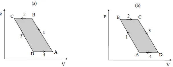
Figure 3.2: Schematic pV-diagram for the thermoacoustic cycle (Fig. (1.4)). a) Refrigerator; the area ABCD represents the work used. b) Prime mover; the area ABCD represents the work produced
The area ABCD represents the work used during the cycle. Actually, the whole gas alongside the wall of the tube contributes to the heat pump process. In Fig.(3.1c), the heat generation of sound in the so-called prime mover, is illustrated. The prime-mover cycle also consists of two adiabatic (1, 3) and two isobaric heat-transfer steps (2, 4). The only difference with the heat-pump case is that now we apply a large temperature gradient ∆T along the tube, so that the directions of heat transfer in steps 2 and 4 are reversed. When the parcel of gas is compressed, it warms up, but is still colder that the local wall position. Heat then flows from the wall into the parcel which expands. As a consequence of this expansion of the gas the piston will be pushed to the left and work is generated. In step 4, after the expansion, the gas element is warmer than the wall and heat flows into the wall. The gas contracts and work is done by the piston. The net work produced in one cycle is given by the area ABCD in Fig. (3.2b). As a result, a standing wave can be sustained by a large temperature gradient along the wall of the tube. In summary, during the compression step 1, the parcel of gas is both displaced along the wall and compressed. Two temperatures are important: the temperature of the gas after adiabatic compression and the local temperature of the wall adjacent to the parcel. If the temperature of the gas is higher than that of the wall, heat flows from the gas to the wall (heat pump). If the temperature of the gas is lower, heat flow sows from wall to gas (prime mover). Both heat flow and power can thus be reversed and the heat transfer process can be switched between the two modes by changing the temperature gradient along the wall. A small temperature gradient is the condition for heat pump; a high gradient is the condition for a prime mover. The gradient that separates the two regimes is called the critical temperature gradient. For this gradient, the temperature change along the wall matches the temperature change due to adiabatic compression, and no heat flows between the gas and the wall. The critical temperature gradient will be summarized in the next section. In the heat-pump regime work is absorbed to transfer heat from lower temperature to higher temperature. In this case, an acoustic wave has to be sustained in the tube to drive the process. In the prime mover mode the gas expands at high pressure (heat absorption), and contracts at low pressure (heat release), so that work is produced. In this case, the large temperature gradient sustains the acoustic oscillations. All periodic heat engines and refrigerators need some time phasing to operate properly. Conventional systems use pistons to compress and displace the gas in a given sequence. In thermoacoustic devices, this time phasing is ensured by the presence of the two thermodynamic media: gas and a solid surface, so that the irreversible heat transfer in steps 2 and 4 introduces the necessary time lag between temperature and motion. The compression and displacement are determined by the acoustic wave instead of pistons. At this stage, it is important to note that not all the gas in the tube is equally effective to the thermoacoustic effect. The elements of gas far away from the wall have no thermal contact, and are simply compressed and expanded adiabatically and reversibly by the sound wave. Elements that are too close to the wall have a good thermal contact, and are simply compressed and expanded isothermally. However elements at about a distance of a thermal penetration depth δk from the wall, have sufficient thermal contact to exchange some heat with the wall and produce a time delay between motion and heat transfer which is necessary for the heat pump process. The quantity δk is the distance across which heat can diffuse through the gas in a time 1/πf, where f is the acoustic frequency.
[image:5.612.170.489.609.705.2]As indicated in section II, Carter et al. realized that the performance of the thermoacoustic Sondhauss tube could be greatly improved by inclusion of a stack of small tubes. This has the effect of increasing the effective contact area between gas and solid over the cross-section of the tube, so that the whole gas contributes to the process. The appropriate use of stacks and their position in acoustically resonant tube scan produce powerful refrigerators (heat pump) and heat engines. We have to note here that even though the system uses a standing wave to displace, compress and expand the gas in the stack, a small travelling acoustic wave component is necessary to maintain the standing-wave resonance against the power absorption in the system. Systems using only traveling waves, which can be made more efficient, are also possible.
IV. APPLICATIONS
In previous section, the essentials of thermoacoustics were explained. Under favorable conditions, powerful or small size thermoacoustic devices can be built to operate as prime-movers or heat-pumps. Since the development of the first practical thermoacoustic apparatus in the early eighties at LANL, thermoacoustic technology has received an increasing attention as a new research area in heat engines and heat pumps. Since then, many thermoacoustic systems have been built, mostly at LANL, Naval Postgraduate School (NPS) in Monterey (California), and at Pennsylvania State University. Heat pumps and refrigerators use an acoustic driver (loudspeaker or prime mover)to pump heat from a cool source to a hot sink. A simple thermoacoustic refrigerator is shown in Fig.1.6. Such systems contain a loudspeaker, which drives an intense sound wave in a gas-filled acoustical resonator. A structure with channels, called the stack is appropriately placed in the tube. The stack is the heart of the refrigerator where cooling takes place. Two examples of refrigerators that were built and tested at NPS are: The Space Thermoacoustic Refrigerator (STAR), which was designed to produce up to 80K temperature difference over the stack, and to pump up to 4 watt of heat. The STAR was launched on the space shuttle Discovery in 1992. The second setup is the Shipboard Electronics Thermo Acoustic Cooler (SETAC) that was used to cool radar electronics on board of the warship USS Deyo in 1995. It was designed to provide 400watt of cooling power for a small temperature span, which is similar to a domestic refrigerator/freezer system. At Pennsylvania State University, a large chiller called TRITON is being developed to provide cooling for Navy ships. It is intended to produce a cooling power of about 10 kW which means that it can convert three tons of water at 00C to ice at the same temperature in one day. At LANL, a heat-driven thermoacoustic refrigerator known as the beer cooler was built, which uses a heat-driven prime mover instead of a loudspeaker to sound necessary to drive the refrigerator. A similar device, called a Thermoacoustic Driven Thermo Acoustic Refrigerator (TADTAR) was recently built at NPS. It has a cooling power of about 90 watt for a temperature span of 25 0C. Such a device has no moving parts at all. Also at NPS, a solar driven TADTAR has been built which has a cooling capacity of 2.5 watt for a temperature span of 17.7 0C At LANL, much of the efforts focused primarily on large thermoacoustic engines, using heat to generate sound, which is used to generate electrical power or to drive coolers to liquefy natural gas. One example of such efforts is collaboration between LANL and an industrial partner to develop a cryogenic refrigeration technology called Thermo Acoustically Driven Orifice Pulse Tube refrigeration (TADOPTR). This technology has the unique capability of producing cryogenic temperatures (115 K) with no moving parts. It uses a pulse-tube refrigerator which is driven by a natural-gas-powered thermoacoustic prime mover. A machine with a cooling capacity of 2kW producing about 0.5 m3/day, has been developed. A second system, using a traveling wave prime mover, is now under construction. This has a higher efficiency, and a cooling capacity of about 140 kW. It is expected that it will burn 20 % of natural-gas to liquefy the other 80 % at a rate of about 50 m3/day. At Tektronix, a TADOPTR was also built to provide cooling of electronic components. The prime mover, used in this cooler, provided 1 kW to the pulse-tube refrigerator with an efficiency of about 23% of Carnot. The prime mover was driven by an electric heater. Hence the system had no moving parts. The potential of applications of thermoacoustic devices is substantial, as can be understood from the foregoing examples. Prime movers can be used to generate electricity, or to drive refrigerators. Thermoacoustic heat pumps can be used to generate heating, air-conditioning or cooling of sensors, supercomputers, etc. Their advantage is that they can have one (loudspeaker) or no moving parts no tight tolerances, making them potentially reliable and low cost. Besides being reliable, they use only inert gases (no CFC.s) so they are environmentally friendly. On the other hand, standing-wave thermoacoustic devices have a relatively low efficiency. However, thermoacoustics still a young technology. Recently, the LANL team has designed a traveling-wave prime-mover which has efficiency much higher than the standing-wave counterpart. This engine is a Stirling version of the thermoacoustic prime-mover. It has a thermal efficiency of 30 % while typical internal combustion engines are 25 to 40% efficient. Thermoacoustic refrigerators can also be made using this principle, and reach efficiencies comparable to vapor compression systems. Swift gave an excellent review of the current status of the field of thermoacoustics in his introductory book .
V. BASIC THERMODYNAMIC AND ACOUSTIC CONCEPTS
V.I. THERMODYNAMIC PERFORMANCE
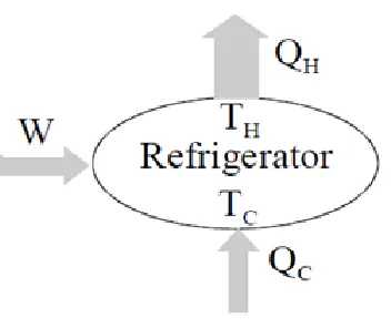
In this section the thermal efficiency for prime movers and the coefficient of performance for refrigerators and heat pumps are introduced, using the first and second law of thermodynamics. From the thermodynamic point of view, prime movers are devices that, per cycle, use heat QH from a source at a high temperature TH and reject waste heat to a source at a lower temperature TC, to generate work W. On the other hand, refrigerators and heat pumps are devices that use work W to remove heat QC at a temperature TC and reject QH at a higher temperature TH. These devices are illustrated in Fig.(5.1).
The energy flows into and out of thermodynamic systems are controlled by the first and second law of thermodynamics. The first law of thermodynamics is a statement of the energy conservation: the rate of increase or decrease of the internal energy U of a thermodynamic system of volume V equals the algebraic sum of the heat flows, and enthalpy flows into the system, minus the work done by the system on the surroundings;
[image:7.612.209.385.219.367.2]̇ ̇ ̇ ̇ (5.1)
Figure 5.1: Representation of a refrigeration of a refrigerator while exchanging per cycle heat and work with the surroundings. The directions of heat and work exchanged between the refrigerator and its environment are shown by the shaded arrows. In a prime mover
the directions of the arrows are reversed.
where ̇ is the molar flow rate of matter flowing into the system, Hm is the molar enthalpy, and P represents other forms of work done on the system. The summations are over the various sources of heat and mass in contact with the system; transfers into the system are positive and those out of the system are negative. The second law of thermodynamics limits the interchange of heat and work in thermodynamic systems. This law states that the rate of change of entropy of a thermodynamic system is equal to the algebraic sum of the entropy change due to the heat flows, due to the mass flow, and due to the irreversible entropy production in the system [1]
̇ ̇ ̇ (5.2)
where the summation is over the various sources with the same sign convention as stated above. The heat flow, ̇, into or out of the system, takes place at the temper-ature T. In addition the second law of thermodynamics requires that
̇ (5.3)
In the following the first and second law of thermodynamics, Eqs.(5.1)-(5.3), will be used to define the performance for refrigerators, heat pumps and prime movers.
V.I.I. REFRIGERATORS AND HEAT PUMPS
The duty of a refrigerator or heat pump is to remove a heat quantity Qc at a low temperature TC and to supply a heat quantity QH to the surroundings at a high temperature TH. To accomplish these processes a net work input, W, is required. This process is illustrated in Fig.(5.1). Refrigerators and heat pumps have different goals. The goal of a refrigerator is to maintain the temperature of a given space below that of the surroundings. While the goal of a heat pump is to maintain the temperature of a given space above that of the surroundings. Since refrigeration and heat pump systems have different goals, their performance parameters, called coefficient of performance (COP) are defined differently. By considering the refrigerator illustrated in Fig.(5.1) and using the fact that there is no mass flow into or out of the system, the first and second law, Eqs.(5.1) and (5.2),take the simple form
̇ ̇ ̇ ̇ (2.4)
And
Where U and S are the internal energy and entropy of the system, respectively; Si is the irreversible entropy production in the system. The integration over one cycle of Eqs.(5.4) and (5.5), and the use of the fact that U and S are functions of state which do not change over one cycle, yields
̇ (5.6)
And
̇ (5.7)
V.I.I(A). REFRIGERATOR
In the case of a refrigerator we are interested in the heat removed QC at TC, and the net work used to accomplish this effect, W. The COPref is given by the ratio of the quantities, thus
(5.8)
Substituting Eq.(5.6) into Eq.(5.8) yields
(5.9)
Since Si ≥ 0, Eq.(5.7) gives
(5.10)
Combining Eq.(5.9) with Eq.(5.10) gives
(5.11)
(5.12)
The quantity is called the Carnot coefficient of performance which is the maximal performance for all refrigerators. This COP can be made larger than one if TC> TH/2. The coefficient of performance relative to Carnot’s coefficient of performance is defined as
(5.13)
V.I.I(B). HEAT PUMP
The performance of heat pumps is defined as the ratio of the desired heat, QH, to the net work needed W. For a heat pump we are interested in the heat QH supplied to a given space. Thus the coefficient of performance, COPhp, is
(5.14)
In combination with Eq.(5.6), this gives
(5.15)
This expression shows that the value of the COPhp is always larger than unity. Combining Eq.(5.15) and Eq.(5.10) leads to the expression
(5.16)
The temperature expression on the right is called the Carnot COPhp which is the maximum performance for all heat pumps. The coefficients of performance COPref and COPhp are defined as ratios of the desired heat transfer output to work input needed to accomplish that transfer. Based on the definitions given above, it is desirable thermodynamically that these coefficients have values that are as large as possible. As can be seen from Eqs. (5.11), (5.16), the second law of thermodynamics imposes limits on the performance, because of irreversibility in the system.
V.I.II. EFFICIENCY OF THE PRIME MOVER
Since the prime mover uses heat QH to produce work W the directions of heat and work flows in Fig.(5.1) are reversed. The performance η of a prime mover is defined as the ratio of the produced work (output) and the heat used to produced that work(input), thus
(5.17)
By use of Eq.(5.6), we have
(5.18)
This expression shows that the efficiency of a prime mover is less than one. Since QH is entering the prime mover and QC is flowing out of it, Eq.(5.10) becomes
(5.19)
In a similar way as described above, we can derive the well-known relation
The temperature expression on the right is called the Carnot efficiency, which is the maximal performance for all prime movers.
V.II. THERMODYNAMIC APPROACH TO THERMOACOUSTICS
A simplified picture of the thermoacoustic effect will be given, using only thermo-dynamics and acoustics to explain how a temperature gradient and hence cooling develops across a stack. The discussion in this section is concerned with the derivation of approximate expressions for the critical temperature gradient and the heat and work flows in thermoacoustic devices. The papers of Wheatley and Swift form the basis for the discussion in this section. Most of the matter and illustrations discussed in the previous section will be repeated here for ease of discussion and derivation of thermoacoustic quantities.
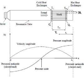
As discussed in the preceding section, thermoacoustic devices consist mainly of an acoustic resonator filled with a gas. In the resonator, a stack consisting of a number of parallel plates, and two heat exchangers, are appropriately installed (Fig.(5.2a)).The stack is the element in which the heat-pumping process takes place. The heat exchangers are necessary to exchange heat with the surroundings, at the cold and hot sides of the stack, as shown in Fig.(5.2a). A loudspeaker sustains an acoustic standing wave in the acoustic resonator. As an approximation, we neglect the viscosity of the gas and the longitudinal thermal conductivity. In response to the acoustic wave, the gas oscillates in the stack channels and is compressed and expanded.
[image:9.612.178.447.346.598.2]We begin by discussing the thermodynamics of a small parcel of gas oscillating along a stack plate, being compressed and expanded by the sound wave. An average longitudinal temperature gradient ∆Tm along the stack is supposed to exist. Addition-ally, we suppose that the pressure antinodes is to the right of the plate and a node to the left (Fig.(5.2b)). For simplicity, the following treatment will assume an in viscid ideal gas of vanishing Prandtl number The four steps of the thermoacoustic cycle are illustrated separately in Fig.(5.3).
Figure 5.2: Model of a thermoacoustic refrigerator. (a) An acoustically resonant tube containing a gas, a stack of parallel plates and two heat exchangers. An acoustic driver is attached to one end of the tube and the other end is closed. Some length scales are also shown: the gas excursion in the stack x1, the length of the stack Ls, the position of the stack from the closed end xs and spacing in the
stack 2 k. b) Illustration of the standing wave pressure and velocity in the resonator.
We suppose that, in the start of the cycle, the temperature, pressure, and volume of the parcel are Tm – x1∆Tm, pm − p1, and V. In step 1, the parcel of gas moves a distance 2x1, is compressed and increases in temperature by an amount 2T1. The adiabatic Pressure change p1 and temperature change T1 are related by the thermodynamic relationship,
( ) (5.21)
( ) (5.22)
where
( ) (5.23)
The subscript m indicates that we are concerned with the mean value of the quantities between brackets. The parameter β is the isobaric volumetric expansion coefficient. Considering an ideal gas (βTm = 1) and using the ideal gas law, the expression (5.22) becomes
( ) (5.24)
[image:10.612.191.460.208.483.2]where γ is the ratio of isobaric to isochoric specific heats.
Figure 5.3: a) Typical gas parcel in a thermoacoustic refrigerator passing through a four-step cycle with two adiabats (step 1 and 2) and two constant-pressure heat transfer steps (2 & 4). B) an amount of heat is shuttled along the stack plate from one parcel of gas to another, as a result Q is transported from the left end of the plate to the right end, using work W. the heat increases in the stack from
Qc to Qh.
After the displacement and compression in step 1, the temperature, pressure and volume becomes Tm−x1∆Tm+2T1, pm+p1, and V –V1. At this time, the temperature difference between the plate and the parcel of gas is
∆ (5.25)
where 2x1∆Tm is the temperature change along the plate. In step 2, for positive δT, heat δQ flows from the parcel of gas to the plate at constant pressure. The heat that flows out of the parcel is given by
(5.26) where m is the mass of the parcel of gas.
In Fig.(5.4), a schematic pV -diagram of the cycle is shown. The work used in the cycle is equal to the area ABCD, and given by
∫ (5.27)
The used acoustic power in each step is shown in Fig.(5.4). Using the acoustic approximation, p1, pm, and the Poisson’s law for the two adiabatic steps, the result after calculation is
(5.28)
The volume δV is related to δT by Eq.(5.23),
( ) (5.29)
Insertion into Eq.(5.28) yields
Figure 5.4: Schematic pV-diagram of the thermoacoustic cycle of Fig.(2.3). the four steps of the thermoacoustic cycle are illustrated: adiabatic compression (1), isobaric heat transfer (2), adiabatic expansion (3) and isobaric heat transfer (4). The area ABCD is the
work used in the cycle which is also egal to the different steps.
In step 3, the parcel of gas moves back to its initial position, expands and cools. At this time, the parcel of gas is colder than the local stack surface, and heat δQ flows into the parcel (step 4).In case δT is negative, heat flows into the parcel which expands and does work δW on its surroundings (prime mover). The sign of the temperature difference δT(and hence magnitude of ∆Tm) determines, after displacement and compression, the direction of the heat flow, into or out of the parcel of gas. Therefore, the refrigerator mode and prime mover mode can be distinguished by the sign of δT. If the temperature change 2x1∆Tm in the plate just matches the adiabatic temperature change 2T1, then the temperature gradient in the stack is named the critical temperature and is given by
(∆ ) (5.31)
Using Eq.(5.22) and x1 = u1/ω, where u=1 is the gas particles velocity amplitude and ω the angular frequency, we obtain
(∆ ) (5.32)
The two modes of operation are characterized in terms of the ratio of the temperature gradient along the stack and the critical temperature gradient
(∆ )∆
(5.33)
Employing Eqs.(5.33), (5.22) and assuming an ideal gas (βT = 1) we can rewrite Eqs.(5.26) and (5.30), as
( ) (5.34)
And
( ) ( ) (5.35)
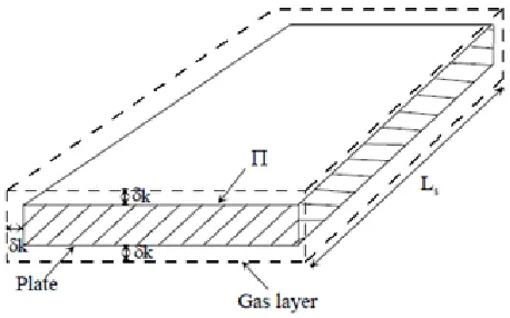
respectively. As can be seen from Fig.(5.5), if we suppose that Π is the perimeter of the plate in the direction normal to the axis of the resonator, Ls is the length of the plate parallel to the resonator axis (wave direction), and since only the layer of gas at a distance δk from the plate contributes to the thermoacoustic heat transport, the effective volume rate of flow of the gas is Πδku1. Here u1 is the amplitude of the speed of motion of the gas, caused by the sound wave.
The thermoacoustic heat flow rate along the plate from TC to TH (refrigerator mode) is obtained by replacing V in Eq.(5.34) by the effective volume flow Πδku1, i.e.
̇ ( ) (5.36)
The total volume of gas that is thermodynamically active along the plate is ΠδkLs, so that the total work used to transport heat is given by
Figure 5.5: A single stack plate at length Ls and perimeter . The gas layer at a distance k from the plate is shown by dashed line. The gas area is equal to k and the total volume of gas in contact with the plate is k Ls.
The power needed to pump the heat is the work per cycle times the frequency ω, so that
[image:12.612.166.465.322.437.2]̇ ( ) (5.38)
Figure 5.6: illustration used in the derivation of the heat conduction equation
When use is made of the definition of the speed of sound and the ideal gas law,
( ) (5.39)
where γ − 1 is the work parameter of the gas, we can rewrite Eq.(5.38) as
̇ ( ) ( ) (5.40) A quantitative evaluation of Q and W for sinusoidal p1 and u1would give the same results except that each expression has a numerical prefatory of 14 . The total heat flow and absorbed acoustic power in the stack can be obtained by using the total perimeter of the plates Πtot instead of the perimeter of one plate Π.
Expressions (5.36) and (5.38) change sign as Γ passes through unity. Three cases can be distinguished: Γ = 1, there is no heat flow and no power is needed; When Γ < 1, the heat is transported against the temperature gradient so that external power is needed, and the device operates as a refrigerator; Γ > 1, due to the large temperature gradient, work is produced, and the device operates as a prime mover. Therefore, the device can operate as a refrigerator as long as the temperature gradient over the plate (stack) is smaller than the critical temperature gradient (Eq.(5.31)).But we can impose a large temperature gradient over the plate so that the device Operates as a prime mover (Γ > 1).
As stated previously, the thermoacoustic effect occurs within the thermal penetration depth δk, which is roughly the distance over which heat can diffuse through the gas in a time 1/πf, where f denotes the frequency of the acoustic wave. In Fig.(5.6),the heat conduction in one dimension through a rod of cross-section A is illustrated. Considering the energy balance for a small element dx of the rod, we suppose that heat is the only form of energy that enters or leaves the element dx, at x and x+dx, and that no energy is generated inside the element. Energy conservation yields
̇
(5.41)
̇ (5.42)
Where Ks is the thermal conductivity of the material. Substituting Eq.(5.42) and the thermodynamic expression du = csdT for the internal energy of solid-state material into Eq.(5.41) yields
(5.43)
where cs and ρs are the isobaric specific heat and density of the material, respectively. If we substitute the characteristic dimensions δs = x/x0 and t0 = ωt into Eq.(5.43) we
Get
( ) (5.44)
so that
( )
(5.45)
and hence
√ (5.46)
where κs is the thermal diffusivity, κs = Ks/ρscs. A similar procedure can be used to derive an analogous expression for the thermal penetration in a gas. Closely related to the thermal penetration depth is the viscous penetration depth in a gas δν. It is roughly the distance over which momentum can diffuse in a time 1/πf and it is given by
√ (5.47)
where the kinematic viscosity ν is given by
(5.48)
here η is the dynamic viscosity of the gas. An important parameter for the performance of thermoacoustic devices is the Prandtl number σ, which is a dimensionless parameter describing the ratio of viscous to thermal effects
( ) (5.49)
For most gases (air, inert gases) but not gas mixtures, σ is nearly 2/3 , so that for these gases thermal and viscous penetration depths are quite comparable. The effect of viscosity on the heat flow and acoustic power will be discussed in the next section.
V.III. ACOUSTIC CONCEPTS
In this section, some acoustic concepts which are important for proper operation of thermoacoustic devices will be described. The discussion will be limited to standing wave thermoacoustic devices, which are more related to the subject of this research.A simple illustration of a thermoacoustic refrigerator is shown in Fig.(5.2). It consists of an acoustic resonator (tube) of length L (along x) and radius r. The resonator is filled with a gas and closed at one end. An acoustic driver, attached to the other end, sustains an acoustic standing wave in the gas, at the fundamental resonance frequency of the resonator. A stack of parallel plates and two heat exchangers are appropriately installed in the resonator.The first condition for the proper operation of thermoacoustic refrigerators is that the driver sustains an acoustic wave. This means that the driver compensates for the energy absorbed in the system. Hence, a small travelling wave component is superimposed on a standing wave; we have to note that in a pure standing wave there is no energy transport.
To illustrate the acoustics, we consider for simplicity that the stack and the heat exchangers have no effect on the acoustic field in the tube. The driver excites a wave along the x direction. The combination of a plane traveling wave to the right and there affected wave at the closed end of the tube generates a sinusoidal standing wave. The acoustic pressure in the tube is given by
( ) ( )
( ) (5.50)
Where p0 is the pressure amplitude at the pressure antinodes of the standing wave, ω is the angular frequency of the wave, k is the wave number. By integration of Newton’s second law (acoustic approximation), ρ ∂u/∂t = −∂p/∂x, thegas particle velocity is
( ) ( )
( ) (5.51)
where
(5.52)
From the fact that sin kx is zero where cos kx is maximum and vice versa, it follows that pressure antinodes are always velocity nodes and vice versa; the pressure and velocity are spatially 90 degrees out-of-phase.
(5.53) Hence,
( ) (5.54)
Where
(5.55)
In this case we see that the first (fundamental) mode which is usually used in thermoacoustic devices, corresponds to L = λ/2, ergo the name half-wavelength resonator. For a quarter-wavelength resonator, one end is open and the other end is closed. This requires a pressure node at the open end, hence
(5.56) So that
( ) (5.57)
The fundamental mode corresponds to L = λ/4, ergo the name quarter-wave resonator. The refrigerator shown in Fig.(5.2), is assumed to be a half-wavelength device. Thus, in the resonance tube, we obtain the pressure and velocity distributions indicated in Fig.(5.2b).
V.IV. BASIC OPERATION CONCEPTS
In the previous sections some basic thermodynamic and acoustic concepts have been introduced. In this section, we will illustrate the effect of the position of the stack in the standing-wave field on the behavior of the thermoacoustic devices .In Fig.(5.2), some important length scales are also shown: the longitudinal lengths, wavelength λ = 2L, gas excursion x1, stack length LS, and the mean stack position from the pressure antinode xS, and the transversal length: spacing in the stack 2δk.For audio frequencies, we have typically for thermoacoustic devices:
(5.58)
Since the sinusoidal displacement x1 of gas parcels is smaller than the length of the plate Ls, there are many adjacent gas parcels, each confined in its cyclic motion to a short region of length 2x1, and each reaching the extreme position as that occupied by an adjacent parcel half an acoustic cycle earlier (Fig.(5.3b)). During the first half of the acoustic cycle, the individual parcels move a distance x1
toward the pressure antinodes and deposit an amount of heat δQ at that position on the plate. During the second half of the cycle, each parcel moves back to its initial position, and picks up the same amount of heat, that was deposited a half cycle earlier by an adjacent parcel of gas. The net result, is that an amount of heat is passed along the plate from one parcel of gas to the next in the direction of the pressure antinode as shown in Fig.(5.3b).
Finally, we note that, although the adiabatic temperature T1 of a given parcel maybe small, the temperature difference ΔTm over the stack can be large, as the .number of parcels., Ls/x1, can be large (Fig.(5.3b)). As from Eq.(5.33)
we find
(∆ )∆
(5.59)
We find
(5.60)
Since Γ < 1, and Ls À x1, we see that ΔTm can be made much larger than T1.
V.IV.I. TEMPERATURE GRADIENT The gas harmonic excursion, x1 is given by
(5.61)
Hence, close to a pressure antinode (velocity node) the excursion of a typical parcel of gas is small. At the same time the parcel experiences large changes in pressure and a large adiabatic temperature change T1 (Eq.(5.22)). So, the critical temperature gradient at that position (∆T)crit = T1/x1 is large. If we replace u1 by its expression
from Eq.(5.51), we get
(5.62)
Using Eq.(5.58) yields
(5.63)
Substituting this result into Eq.(5.31)we obtain
( ) ( ) (5.64)
V.IV.II. HEAT FLOW
Eq.( 5.36) shows that the heat flow is proportional to the product p1u1, and so vanishes if the stack is placed at either a pressure node or a velocity node of the standing acoustic wave. The maximum value of p1u1is at x = λ/8 = L/2. The factor (Γ − 1) appears also in the expression of heat flow. This factor is negative for refrigerators, and its effect can be derived from the discussion in preceding subsection. The lateral section of gas effective for the process Πδk, can be maximized by using more plates, optimally spaced, in the stack so that the total perimeter Π is as large as possible while maintaining a stack spacing greater than about 2δk .
V.IV.III. ACOUSTIC POWER
In the absence of viscosity, the expression for the power needed to pump heat, Eq.(5.40), is similar to that of heat flow, the only difference is the presence of the work parameter (γ − 1). Since each parcel along the plate absorbs net work, the total work done on the gas is proportional to the plate length Ls.
V.IV.IV. VISCOSITY
The discussion above concerns and in viscid gas. When viscosity is taken into account, the resulting expressions are much more complicated. These expressions will be presented in the following chapter.The viscous penetration depth is nearly as large as the thermal penetration depth, so most of the gas in the stack experiences significant viscous shear. However, the definition of the critical temperature gradient (Eq.(5.32)) will be kept throughout this thesis. In fact, with viscosity present, there is a lower critical temperature gradient below which the engine pumps heat and a higher critical gradient above which the engine is a prime mover. Between these two limiting gradients the engine is in a useless state, using work to pump heat from hot to cold.
V.IV.V. PERFORMANCE
At this stage, an estimation of the theoretical performance of the thermoacoustic devices, using an inviscid working gas, can be calculated from the expression of COP(η) derived in previous section in combination with the heat and work equations the COP is given by
̇ ̇ (5.65)
Making use of Eqs.(5.32), (5.36), (5.38) and ΔTm = TmLs yield
(5.66)
Here COPC is Carnots coefficient of performance (Eq.(5.11)), the maximum possible performance of a refrigerator at Tm spanning the temperature difference ΔTm. We see that COPC is approached as Γ → 1, in which case heat and work are zero.
We note that standing-wave thermoacoustic devices are intrinsically irreversible. The irreversible heat transfer δQ across the temperature difference δT, steps 2 and 4 in Fig.(5.3), is essential to the operation of these devices. They do rely on the imperfect thermal contact across the thermal penetration depth δk, which provides the necessary phasing between displacement and thermal oscillations. This is the reason why the performance of standing wave thermoacoustic devices falls below Carnot performance. The performance will be degraded furthermore if viscous, thermal conduction and other losses in the different parts of the device will be considered. To date, the best performance reached with such devices is about 20 % of Carnot.
VI. THEORY OF THERMOACOUSTICS
Although thermoacoustic phenomena are experimentally observed for over two centuries, it is only during the seventies that the general linear thermoacoustic theory has been developed by Rott and coworkers. The theory was first developed for heat generated oscillations (prime mover), but it is also applicable to thermoacoustic refrigerators and heat pumps. In this chapter the Rott’s theory of thermoacoustics will be presented.
VI.I. GENERAL THERMOACOUSTIC THEORY
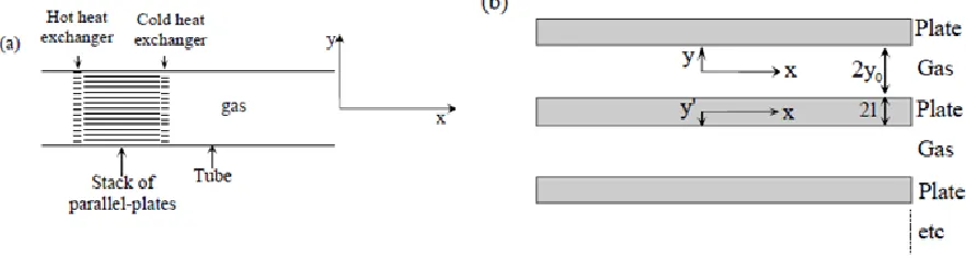
The thermoacoustic theory as known today is first developed by Rott and reviewed later by Swift. Starting with the linearization of the Navier-Stokes, continuity, and energy equations, we will proceed to develop the thermoacoustic equations avoiding much of the detail which has been provided elsewhere. For extended and detailed derivation of the different expressions, reference will be made to more specialized papers. The thermoacoustic equations are three fold: the first equation consists of Rott’s wave equation, which is the wave equation for the pressure in the presence of a temperature gradient along the stack; the energy equation, which describes the energy flow in thermoacoustic systems; and the third equation that is an expression for the acoustic power absorbed (refrigerator) or produced (prime mover) in the stack. We will follow the notation used by Swift .The geometry used to derive and discuss the thermoacoustic equations is illustrated in Fig.(6.1). We consider a parallel-plate stack placed in a gas-filled resonator. The plates have a thickness 2l and gas spacing 2y0. The x axis is along the direction of acoustic vibration and the y axis perpendicular to the planes of the parallel plates,with y = 0 in the center of the gas-layer and y = y0 at the gas-solid boundary. An y0 axis is considered for the plates, with y0 = 0 in the center of the plate and y0 = l at the boundary. So there are two opposite coordinate systems as indicated in Fig.(6.1).
The theory is linear, second-order effects other than energy transport, such as acoustic streaming and turbulence are neglected.
The plates are stationary and rigid.
The temperature spanned along the stack is much smaller than the absolute temperature.
The temperature dependence of viscosity is neglected, which can be important at large temperature gradients. Oscillating variables have harmonic time dependence at a single angular frequency ω.
[image:16.612.87.528.177.295.2]We note that sound results from a time-varying perturbation of dynamic and thermodynamic variables that describe the medium. a one-dimensional acoustic wave with an angular frequency ω exists, and the acoustic pressure is constant over the cross-sectional area of the stack, so that p = p(x).
Figure 6.1: Geometry used for the derivation of thermoacoustic expressions. (a) Overall view, and (b) expanded view of the stack section. Each plate has thickness el, and each gas layer has thickness 2y
In thermoacoustics, a first order in the perturbations is considered for variables, and a second order in the perturbations for the energies. The fundamental physics concerned with thermoacoustics is described by Navier-Stokes continuity and energy equations
[ ( ) ] ( ) ( ) (6.1)
( ) (6.2)
( ) [ ( ) ] (6.3)
where ρ is density, v is velocity, p is pressure, µ and ξ are dynamic (shear) and second(bulk) viscosity, respectively; K is the gas thermal conductivity, and h are internal energy and enthalpy per unit mass, respectively, and Σ is the viscous stress tensor with components
(
)
(6.4)
The temperature in the plates is given by the conduction equation
(6.5)
where Ks, ρs and cs are the thermal conductivity, the density and specific heat per unit mass of the stacks material, respectively. The temperature in the fluid is given can be derived from Eq.(6.3)
( ) ( ) (6.6)
The temperatures in the plates and in the gas are coupled at the solid-gas interface where continuity of temperature and heat fluxes is imposed. These conditions are respectively expressed as
( ) ( ) (6.7)
K ( ) (
)
where subscript 1 indicates a first-order in the perturbation. The complex notation is used for time-oscillatory variables: pressure p, temperature T, velocity components (u, v,w), density ρ, and entropy per unit mass s
[ ( ) ] (6.8)
[ ( ) ] (6.9)
(6.10)
( ) [ ( ) ] (6.11)
(6.12)
variables. Since δν, and λ are the characteristic lengths in x, y directions, respectively, and δν<<λ. This means that through this section we will always neglect ∂/∂x compared to ∂/∂y. To first order, the x-component of the momentum equation can be written in the form
( ) ( ) (6.13)
where u1 is the x component of v1. Thus Eq.(6.13) reduces to
(6.14)
With the boundary condition u1(y0) = 0, the solution u1 of this equation can be written as the sum of the solution of the homogenous equation and a particular solution. The solution is
( ) ( ) [ [ ( ) ] [( ) ] ] (6.15) Where √ (6.16)
The parameter δν is the viscous penetration depth of the gas as defined in chapter 2.To first order, Eq.(6.5) becomes
(6.17)
Using the first boundary condition from expression (6.7), Eq.(6.17) has the solution
( ) ( )[
( ) (
) ( )]
( )
( ) (6.18)
Where
( )
( ) (6.19)
( ) ( ) √ √ ( ) ( ) ( ) And
√ (6.20)
√ (6.21)
( ) (6.22)
where δk is the thermal penetration depth of the gas, δs is the solids thermal penetration depth, and σ is the Prandtl number. The function f is the so called Rotts function and it is geometry dependent. Using the thermodynamic expression
( ) ( ) (6.23)
where cp and β are the specific heat per unit mass and the isobaric thermal expansion coefficient of the gas, respectively. To first order, Eq.(6.6) becomes
( )
(6.24)
Substituting Eq.(6.15) for u1, and solving Eq.(6.24) for T1, with the boundary condition of Eq.(6.7). The solution is
( ) ( [( ) ( ) ( )]) ( ( ) ( ) ) ( ) ( ) ( ) ( ) For the derivation of Rott’s wave equation, we begin with the continuity equation, Eq.(6.2), which to first order becomes
( ) (6.25)
By combining this equation with the x derivative of Eq.(6.14), one obtains
(
)
(6.26)
( ) (6.28)
where γ is the ratio of isobaric to isochoric specific heats and a is the adiabatic sound speed. Substituting Eq.(6.28) into Eq.(6.27), yields ( ) (6.29)
By incorporating Eqs.(6.25) and (6.15) into Eq.(6.29), and integrating with respect to y from 0 to y0, we obtain the wave equation of Rott
[ ( ( )) ] [( ) ] ( )( ( ) ) (6.30)
This is the wave equation for p1 in the presence of a mean temperature gradient dTm/dx in the stack. For an ideal gas and ideal stack with
ε
s = 0, this result was first obtained by Rott. Now, we will proceed to develop an expression for the time-averaged acoustic power dW used (or produced in the case of a prime mover ) in a segment of length dx in the stack. This power is the difference between the average acoustic power at x+dx and x, thuṡ [( ̅̅̅̅̅̅̅̅̅) ( ̅̅̅̅̅̅̅̅̅) ] (6.31)
where over bar indicates time average, brackets indicate averaging in the y direction, and Ag is the cross-sectional area of the gas within the stack. Expanding ( ̅̅̅̅̅̅̅̅̅) in a Taylor series, and p being independent of y, Eq.(6.31) can be written as
[ ( )̅̅̅̅̅̅̅̅ ] (6.32)
The time average of the product of two complex quantities such as p1 and u1 is given by
( )
̅̅̅̅̅̅̅̅̅ [ ( ̇ )] (6.33)
where the star denotes complex conjugation and signifies the real part. Using Eq.(6.33) and expanding the derivatives in Eq.(6.32) gives
̇ [ ( ̇ ) ( ̇ ) ] (6.34)
To evaluate this expression, the derivatives dp1/dx and ( ̇ )
are needed. The expression for dp1/dx is obtained from Eq.(6.15), as follows
( )
( ) (6.35)
so that
( )
( ) (6.36)
The derivative dp1/dx can be obtained from the second term in Rott’s wave equation and Eq.(6.35), as follows
[
( )
] ( ( )) (6.37)
Substituting this into Eq.(6.30) produces ( )
[ ( ( )) ] ( )( ( )( ) ) ( ) (6.38) Substituting Eqs.(6.36) and (6.38) into Eq.(6.34) yields
( ( ) | | |( )| ( ) ( ) ( ) | | ) ( ( )( ) ( ( )
( ) ( ))) (6.39)
This is the acoustic power absorbed (or produced) in the stack per unit length. The subscript 2 is used to indicate that the acoustic power is a second-order quantity; the product of two first-order quantities, p1 and u1.
The first two terms in Eq.(6.39), are the viscous and thermal relaxation dissipation terms, respectively. These two terms are always present whenever a wave interacts with a solid surface, and have a dissipative effect in thermoacoustics. The third term in Eq.(6.39) contains the temperature gradient dTm/dx. This term can either absorb (refrigerator) or produce acoustic power (prime mover) depending on the magnitude of the temperature gradient along the stack. This term is the unique contribution to themoacoustics.
Finally, we will now proceed to develop an expression for the time-averaged energy Flux E2 in the stack, correct to second-order in the acoustic variables. We consider the thermoacoustic refrigerator shown in Fig(6.1a), driven by a loudspeaker. We suppose that the refrigerator is thermally insulated from the surroundings except at the two heat exchangers, so that heat can be exchanged with the outside world only via the two heat exchangers. Work can be exchanged only at the loudspeaker piston. The general law of conservation of energy for a fluid, where there is viscosity and thermal conduction is given by Eq.(6.3), is expressed by Eq.(6.40) below
( ) [ ( ) ] (6.40)
the divergence of the energy flux density which consists of three terms: transfer of mass by the motion of the fluid, transfer of heat and energy flux due to internal friction, respectively.
In steady state, for a cyclic refrigerator (prime mover) without heat flows to the surroundings, the time averaged energy flux E2 along x must be independent of x. Terms of third order in v are neglected. Taking the x component of Eq.(6.40), integrating the remaining terms with respect to y from y = 0 to y = y0, and time averaging yields
[∫ ̅̅̅̅̅̅ ∫ ̅̅̅̅̅ ∫ ̅̅̅̅̅̅̅̅̅ ∫ ̅̅̅̅ ]
=0 (6.41)
The quantity within the square brackets is the time-averaged energy flux per unit Perimeter E2/Π along x
̇ =∫ ̅̅̅̅̅ ∫ ̅̅̅̅̅ ∫ ̅̅̅̅̅̅̅̅ ∫ ̅̅̅̅ (6.42)
Using the acoustic approximations Eqs.(6.8)-(6.12), keeping terms up to second order the first integral in Eq.(6.42) becomes
̅̅̅̅̅ ̅̅̅ ̅̅̅ ̅̅̅̅̅̅ + ̅̅̅̅̅̅ (6.43)
The first term on the right in Eq.(6.43) is zero because u1 = 0. The integrals of the second and third terms in Eq.(6.43) sum to zero because the second-order time- averaged mass flux is zero
̅̅̅̅̅̅ ̅̅̅=0 (6.44) Hence, if we use the thermodynamic expression
( ) ( ) (6.45)
we obtain
̅̅̅̅̅ ̅̅̅̅̅̅ ̅̅̅̅̅̅ ( ) ̅̅̅̅̅̅ (6.46)
The largest term in the last integral in Eq.(6.42) is of order y0µu1/λ; but the term ρuh, in the first integral, is of order p1u1 ~ ρmau12, so that the last integral can be neglected. Only the zero-order terms are significant in the second and third integrals
in Eq.(6.42). Hence Eq.(6.42) becomes
̇
∫ ̅̅̅̅̅̅ ( ) (6.47)
∫ ̅̅̅̅̅̅ ∫ ̅̅̅̅̅̅ ( ) (6.48) so that ̇ ∫ [ ̅̅̅̅̅̅ ( ) ̅̅̅̅̅̅] ( ) (6.49)
The subscript 2 is again used to indicate that the energy flux is second order in the acoustic quantities. Substituting Eq.(6.15) for u1 and Eq.(6.25) for T1 and performing the integration yields finally
[ 〈 〉 ( ( )( ( )( ) ))]+ |〈 〉| ( )( )| | [ ( )( ) ( )( ) ] [ ] (6.50)
where As is the cross-sectional area of the stack material. This important result represents the energy flux along x direction (wave direction) in terms of Tm(x), p1 (x), material properties and geometry. For an ideal gas and ideal stack
ε
s = 0, this result was first obtained by Rott . As can be seen from Eq.(6.47), the energy flux consists of three terms: the first term in p1u1 is the acoustic power, the second term in s1u1 is the hydrodynamic entropy flow, and the final term is simply the conduction of heat through gas and stack material in the stack region. As discussed before, the time-averaged energy flux ̇ along the stack must be independent of x. With ̇ constant, we solve Eq.(6.50) for dTm/dx, so that Tm can be evaluated{ ̇ [ 〈 〉 ( ( )( ( )( ) ))]} { ( )( |〈 )| 〉| | [ ( )( ) ( )( ) ] } (6.51)
As can be seen from Eqs.(6.39) and (6.50), the expressions for the acoustic energy flows are complicated and difficult to interpret. But they are useful for numerical calculation.
VI.II. BOUNDARY LAYER AND SHORT-STACK APPROXIMATIONS
The thermoacoustic expressions derived in the previous section are complicated to interpret. In this section we will use two assumptions, to simplify these expressions. First, we make use of the .boundary-layer. Approximation: y0>>δK, l >>δs, so that the hyperbolic tangents in Eq.(6.19)can be set equal to unity. Second, we make the short-stack. Approximation, Ls <<λ; where the stack is considered to be short enough that the pressure and velocity in the stack does not vary appreciably. Finally, we will consider standing-wave systems, which are more related to the experimental work in this study.
The standing wave acoustic pressure in the stack , can be taken as real and is given by
( ) (6.52)
and the mean gas velocity in x direction is
〈 〉 ( ) ( ) 〈 〉 (6.53)
The superscript s refers to standing waves, p0 is the pressure amplitude at the pressure antinodes of the standing wave and k is the wave number. The factor (1+l/y0) is used because of the continuity of the gas volumetric velocity at the boundary of the stack which requires that the velocity inside the stack must be higher than that outside by the cross-sectional area ratio (1 + l/y0). The Rott’s function f in the boundary layer-approximation is given by
( ) (6.54)
Using these assumptions and Ag = Πy0, As = Πl; the approximate expressions for ̇ and ̇ are obtained, respectively.
̇ ( ) ( )
( ) (( √ ) )
〈 〉
(6.55)
And
̇ ( )( 〈 〉) [[ √ √ ( √ )] [ ]
(6.56)
Where
(6.57)
In Eq.(6.55), LS is the stack length, Π is the total perimeter of the stack plates in the direction normal to the x axis, and ΠδkLS is the volume of gas within about a thermal penetration depth from the plates. Γ = Tm/ Tcrit, and Tcrit is given by Eq.(2.32)
〈 〉 (6.58)
The second term on the right hand side of Eq.(6.55) and the second term between brackets (−1) are negative and are the viscous and thermal relaxation dissipation terms, respectively. These two terms have a dissipative effect on the performance of thermoacoustic devices. The first term between brackets on the right hand side of Eq.(6.55), proportional to Γ, is the acoustic power absorbed to transfer heat (Γ < 1)or produced in the case of a prime mover ( Γ > 1). We note again that the acoustic power W2 and energy E2 are quadratic in the acoustic amplitude. Furthermore, W2 is proportional to the volume ΠδkLS of gas that is located within δk from the stack surface.
As will be shown in the next section, the E2 is the heat removed from the cold heat exchanger in our refrigerator. The first term on the right hand side of Eq.(6.56) is the thermoacoustic heat flow. The second term on the right hand side of Eq.(6.56) is simply the conduction of heat through gas and stack material in the stack region. So that the heat conduction has also have a negative effect on the performance of thermoacoustic refrigerators. The energy flow E2 is proportional to the area Πδk, which is the cross- sectional area of gas that is at δk from the stack surface. If δk ~y0, essentially the entire cross-sectional area of gas in the stack participates in the thermoacoustic heat transport. The energy flow is also proportional to the product 〈 〉. Equations (6.55) and (6.56) contain the important parameter Γ which determines the sign of this expressions and hence the mode of operation of the apparatus, as discussed previously. Substituting Eqs.(6.52) and (6.53) into Eq.(6.58), we obtain
( ( )
)
( ) (6.59)
Eq.(6.59), shows that the critical temperature gradient is independent of the acoustic amplitude for a given location of the stack center within the standing wave. We see from Eq.(6.55) and Eq.(6.56), that the energy flow and acoustic power depend on of the Prandtl number σ (viscosity), in a complicated way. The influence of the Prandtl number on ̇ and ̇ and hence on the performance of the refrigerator will be discussed in the next section.
VI.III. ENERGY FLUXES IN THERMOACOUSTIC REFRIGERATOR