University of Huddersfield Repository
Holroyd, GeoffreyThe modelling and correction of ballscrew geometric, thermal and load errors on CNC machine tools
Original Citation
Holroyd, Geoffrey (2007) The modelling and correction of ballscrew geometric, thermal and load errors on CNC machine tools. Doctoral thesis, The University of Huddersfield.
This version is available at http://eprints.hud.ac.uk/id/eprint/2627/
The University Repository is a digital collection of the research output of the University, available on Open Access. Copyright and Moral Rights for the items on this site are retained by the individual author and/or other copyright owners. Users may access full items free of charge; copies of full text items generally can be reproduced, displayed or performed and given to third parties in any format or medium for personal research or study, educational or notforprofit purposes without prior permission or charge, provided:
• The authors, title and full bibliographic details is credited in any copy; • A hyperlink and/or URL is included for the original metadata page; and • The content is not changed in any way.
For more information, including our policy and submission procedure, please contact the Repository Team at: [email protected].
THE MODELLING AND CORRECTION OF BALL-SCREW
GEOMETRIC, THERMAL AND LOAD ERRORS
ON CNC MACHINE TOOLS
GEOFFREY HOLROYD
A Thesis submitted to the University of Huddersfield in partial fulfilment of the
requirements for a degree of Doctor of Philosophy
The University of Huddersfield
ABSTRACT
In the modern global economy, there is a demand for high precision in manufacture as competitive pressures drive businesses to seek greater productivity. This results in a demand for a reduction in the errors associated with CNC machine tools. To this end, it is useful to develop a greater understanding of the mechanisms which give rise to errors in machine tool drives.
This programme of research covers the geometric, thermal and load errors commonly encountered on CNC machine tools. Several mathematical models have been developed or extended which enable a deeper understanding of the interaction between these errors, various details of ballscrew design and the dynamic behaviour of ballscrew driven systems.
Some useful models based on the discrete matter or “lumped mass” approach have been devised. One extends the classical eigenvalue method for finding the natural frequencies and other dynamic characteristics of ballscrew systems to include viscous damping effects using a generalised eigenvalue approach. This gives the damping coefficient of each predicted vibration mode along with the estimates of the natural frequencies, enabling many of the natural frequencies predicted by standard undamped natural frequency analyses to be dismissed as being of little consequence to the vibratory behaviour of the system.
A development of this modelling method gives the sensitivity of the system to changes in stiffness and damping characteristics, which is helpful at the preliminary design stage of a ballscrew system, and is an aid in deciding the most convenient remedy to vibration problems which may occur in service.
The second set of lumped-mass models is specially developed to take account of the changes in the configuration of the system with time as the nut moves along the screw while taking into account the non-linear phenomena of backlash and Coulomb friction. These can deal with the axial, torsional and transverse degrees of freedom of the system and predict many aspects of the dynamic behaviour of a ballscrew system which have an effect on the errors arising from such systems. They also include features which calculate the energy converted to heat by all the energy dissipative mechanisms in the model which can be used in conjunction with models already developed at the University of Huddersfield to predict thermal errors.
ACKNOWLEDGEMENTS
I would like to acknowledge my dept of gratitude for the support I have received during the course of this Research Project.
I am grateful for the funding provided by the ROBCON - EPSRC project 'Robust On-line Parameter Identification and Modelling Applied to a Precision 3-axis Machine Tool for Control and Condition Monitoring Purposes', EPSRC Grant GR/S07827/01.
I would also like to thank the people who have acted as Director of Studies and Supervisors throughout the Project. First Professor Derek Ford, now Emeritus Professor at the University of Huddersfield, for his overall leadership and many helpful and useful comments and suggestions; Dr Mike Freeman for his help and encouragement with the mathematical analysis; Dr Simon Fletcher for his oversight of much of the practical work and his valuable input to the thermal aspects of the work; Dr Crinela Pislaru for her help and advice on various aspects of modelling, especially hybrid modelling, for her collaboration over the aspects relating to measurements taken on a CNC machine then in use at Huddersfield, and her help and advice in preparing this Thesis; Mr Steve Millwood for his help in the early days of programming in C; Dr Veimar Castaneda for his insights into the detailed working of the Heidenhain controller used on the Linear Guide Rig, and the technical support staff for their support in making parts specially required for the experimental work.
Finally, I would like to thank my wife Nora and my children Chloe and Christian for their support and patience over the years.
CONTENTS
ABSTRACT ii
ACKNOWLEDGEMENTS iii
CONTENTS iv
LIST OF FIGURES viii
LIST OF TABLES xii
NOMENCLATURE xiii
CHAPTER 1 – INTRODUCTION 1
CHAPTER 2 - LITERATURE SURVEY 8
2.1 Basic modelling of screw mechanisms 8
2.2 Error compensation in CNC machine tools 9
2.3 Feed drives modelling 14
2.4 Analysis of vibration damping for feed drives 18
2.5 Summary 21
CHAPTER 3 - THEORETICAL BACKGROUND 26
3.1 Basic characteristics of a ballscrew 26
3.2 Errors in machine tool drives 29
3.3 Factors affecting thermal, geometric and load performance 31
3.3.1 Bearings 31
3.3.2 Ball nut 34
3.3.3 Pre-tension 35
3.4 Basic behaviour of screw 35
3.4.1 Ballscrew driving 38
3.4.2 Ballscrew driven 38
3.5 Static elastic theory 39
3.5.1 General Hertzian theory 39
3.5.2 Other elastic effects 43
3.5.3 Rolling element friction 45
3.6 Dynamic elastic theory 46
CHAPTER 4 - DYNAMIC MODEL – GENERAL CONSIDERATIONS 47
4.1 Continuous matter approach – wave solutions 48
4.2 Lumped mass approach – matrix solutions 54
4.3.1 An eigenvalue approach – undamped case 58 4.3.2 A generalised eigenvalue approach – damped case 66
4.3.3 Sensitivity analysis 71
CHAPTER 5 - AXIAL AND TORSIONAL CASE FOR MOVING MASS MODEL 73
5.1 Dynamics of a ballscrew with a moving nut– the axial case 75 5.2 Solution of differential equation with time-dependent coefficients 78
5.3 Extension to include torsional movement 83
5.4 Backlash 87
5.5 A refinement of the method 89
5.6 Comparison with classical theory 95
CHAPTER 6 - TRANSVERSE CASE FOR MOVING MASS MODEL 100
6.1 Modelling the transverse behaviour of the screw 100
6.2 Combining the transverse behaviour of the screw with the axial and torsional 101
6.3 Initial conditions 106
6.4 Developing the transverse motion of the ballscrew system 108
6.5 Gyroscopic effect 111
6.6 Ballscrew orbits 112
6.7 Bearing cap vibrations 113
6.8 Out-of-balance excitation 114
CHAPTER 7 - THERMAL CONSIDERATIONS 116
7.1 Modelling of screw – justification of one dimensional approach 119
7.2 Thermal behaviour of bearings 125
7.3 Thermal behaviour of nut 127
7.4 Ballscrew system thermal model 127
7.5 Ballscrew cooling 129
7.5.1 Cooling using a moving fluid 130
7.5.2 Evaporative cooling 133
7.6 Comparison with measured data 134
CHAPTER 8 - EXPERIMENTAL VERIFICATION 137
8.1 Static measurements 140
8.1.1 Preliminary considerations 141
8.1.2 Measurement strategy 144
8.1.3 Measurement results 146
8.2 Dynamic measurements – nut in fixed position 151
8.2.1 Preliminary considerations 152
8.2.2 Measurement strategy 152
8.2.3 Measurement results 155
8.3 Dynamic measurements – nut moving along screw 156
8.3.1 Preliminary considerations 156
8.3.2 Measurement strategy 156
8.3.3 Measurement results 157
CHAPTER 9 - ERROR REDUCTION 160
9.1 Error reduction through design 160
9.1.1 Effects on stiffness of detailed geometry 160
9.1.2 Thermal considerations 161
9.1.3 Material considerations 161
9.2 Error reduction through compensation 162
9.2.1 Compensation for dynamic effects 162
9.2.2 Compensation for thermal effects 166
CHAPTER 10 – CONCLUSIONS 168
REFERENCES 172
APPENDIX 4.1 – Validation of continuous matter test model 184
APPENDIX 4.2 - Details of Y-axis drive for Beaver VC 35 CNC machine tool 189 APPENDIX 4.3 – MATLAB function for calculating undamped natural frequencies 190 APPENDIX 4.4 – MATLAB function for calculating transverse natural frequencies 194 APPENDIX 4.5 – MATLAB function for calculating damped natural frequencies 198 APPENDIX 4.6 – MATLAB routine for calculating sensitivity of a ballscrew system to
changes in stiffness 204
APPENDIX 4.7 – MATLAB routine for calculating sensitivity of a ballscrew system to
changes in damping 206
APPENDIX 4.8 – MATLAB routine for calculating sensitivity of a ballscrew system to
changes in inertia 209
APPENDIX 5.1 - “C” program for axial and torsional degrees of freedom 212 APPENDIX 5.2 - Details of calculations used to check Program T3 236 APPENDIX 6.1 – C program for 6 degree-of-freedom mechanical model 240
APPENDIX 7.2 – Matlab model “cool2.m” 247
APPENDIX 7.3 – The ballscrew thermal model 248
APPENDIX 7.4 – Mini TK model “BS_COOL1.TK” 262
APPENDIX 8.1 - Static deflection theory – zero pre-tension 263
APPENDIX 8.2 - Static deflection theory – non-zero pre-tension 274 APPENDIX 8.3 – Dynamic behaviour of a shaft under centrifugal forces 285 APPENDIX 8.4 – Data extraction and results – Fixed nut, all positions 288 APPENDIX 8.5 – Data extraction and results – Moving nut, all positions 293
APPENDIX 8.6 - Linear Guide rig – Data 298
LIST OF FIGURES
Figure 2.1 – The essential elements of a typical machine tool drive 16
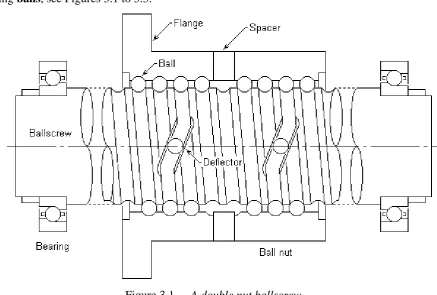
Figure 3.1 - A double nut ballscrew 26
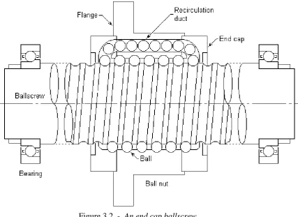
Figure 3.2 - An end cap ballscrew 27
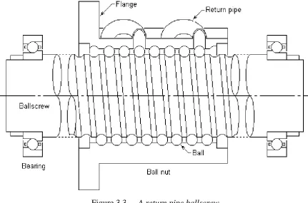
Figure 3.3 - A return pipe ballscrew 28
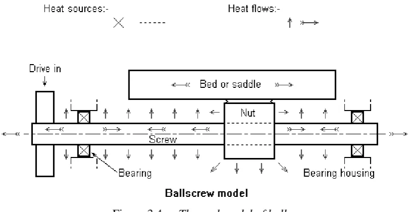
Figure 3.4 - Thermal model of ballscrew 30
Figure 3.5 – The “fixed-free” bearing arrangement 31
Figure 3.6 – The “fixed-supported” bearing arrangement 32
Figure 3.7 – The “fixed-fixed” bearing arrangement 32
Figure 3.8 – The “fixed-fixed” screw clamping arrangement 32
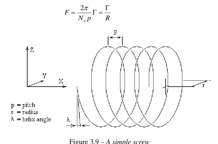
Figure 3.9 – A simple screw 36
Figure 3.10 – “Ballscrew driving” mode of operation 37
Figure 3.11 – “Ballscrew driven” mode of operation 37
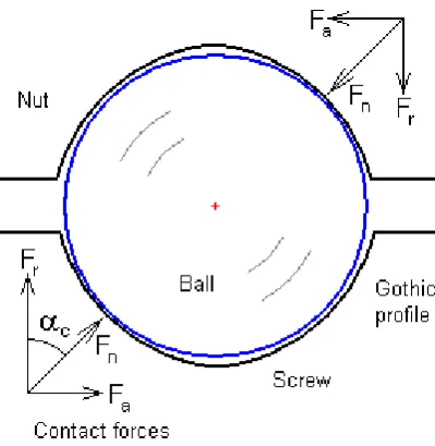
Figure 3.12 – Contact in ballscrew meshing action 41
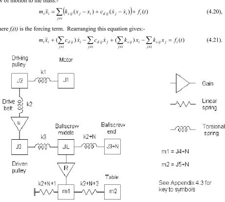
Figure 4.1 - A feed drive system 47
Figure 4.2 - A ballscrew drive system - discrete matter approach 48 Figure 4.3 - A ballscrew drive system - continuous matter approach 49 Figure 4.4 - A test model made of two masses connected by a continuous matter spring 51 Figure 4.5 – A model based on wave theory of two masses connected by a spring 53
Figure 4.6 - Beaver VC35 CNC milling machine 54
Figure 4.7 - Beaver Machine – X or Y drive 55
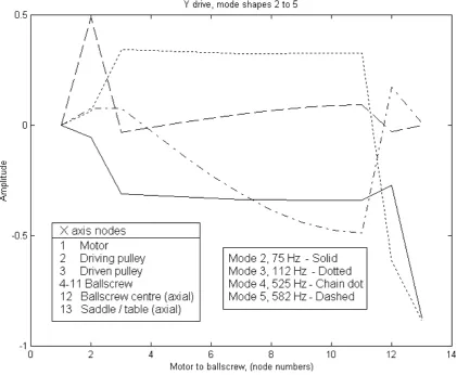
Figure 4.8 - Schematic representation of the mechanical elements of the drive model 56 Figure 4.9 - Undamped mode shapes predicted by the eigenvalue method 62 Figure 4.10 - Natf_tr1.m – Natural frequency and modes shapes – free-free 64 Figure 4.11 - Natf_tr2.m – Natural frequency and modes shapes – fixed-free 65 Figure 4.12 - Natf_tr3.m – Natural frequency and modes shapes – supported-supported 65 Figure 4.13 - Natf_tr4.m – Natural frequency and modes shapes – fixed-fixed 66 Figure 4.14 - Representation of viscous damping phenomenon 67 Figure 4.15 - Model of the mechanical transmission of the CNC machine tool axis drive
considering viscous damping 69
Figure 4.16 - Damped mode shapes predicted by the
generalised eigenvalue method – Cartesian 70 Figure 4.17 - Damped mode shapes predicted by the
generalised eigenvalue method – polar 71
Figure 5.1 - Simple “mass on a spring” system 73
Figure 5.3 - A typical ballscrew in a machine tool drive 76
Figure 5.4 - Ballscrew model 76
Figure 5.5 - Ballscrew system model 85
Figure 5.6 - Ballscrew backlash 87
Figure 5.7 - First method 90
Figure 5.8 - The refined method 90
Figure 5.9 - Comparison with classical theory 95
Figure 5.10 – Ballscrew torsional displacement 96
Figure 5.11 – Ballscrew torsional velocity 96
Figure 5.12 - Ball nut displacement 96
Figure 5.13 - Ball nut velocity 96
Figure 5.14 – Ballscrew axial displacement 97
Figure 5.15 – Ballscrew axial velocity 97
Figure 5.16 – Torque applied at the driven end of the ballscrew 98
Figure 5.17 – Ball nut position error 98
Figure 6.1 The global reference axes 100
Figure 6.2 Six degree of freedom matrix for a beam element
representing part of the ballscrew 103
Figure 6.3 Y and θz degree of freedom matrix for the beam element representing part of the ballscrew in contact with nut
a - Terms in Izz, kn and φn 104
b - Additional terms in kn 104
c - Additional terms in φn 105
d - Additional terms in kn φn 105
Figure 6.4 Axes rotated with ballscrew 108
Figure 6.5 Polar coordinate system 109
Figure 6.6 Gyroscopic effects 111
Figure 6.7 Modelling bearing cap 113
Figure 6.8 Trajectory of ballscrew centre under out-of-balance load 115 Figure 7.1 – A comparison of one-dimensional thermal and two-dimensional
thermal models of a ballscrew, 2Dave – 1D 124
Figure 7.2 – A comparison of one-dimensional thermal and two-dimensional
thermal models of a ballscrew, 2Dsurf – 1D, heating 124
Figure 7.3 – A comparison of one-dimensional thermal and two-dimensional
thermal models of a ballscrew, 2Dsurf – 1D, cooling 125
Figure 7.4 - Heat transfer elements of ballscrew system model 127
Figure 7.5 – Evaporative cooling – typical temperature drop 133
Figure 7.7 – Energy dissipated in nut and bearings – thermal model 135 Figure 7.8 – Energy dissipated in nut and bearings – dynamic model 135 Figure 7.9 - Simulated and measured error between axis positions 0 and -460 during
a heating and cooling cycle 136
Figure 8.1 – Ballscrew linear guide rig with controller
and vibration monitoring equipment 137
Figure 8.2 – Ring used as a target for an N.C.D.T and to carry out-of-balance weights 139
Figure 8.3 Dimensions A and B 141
Figure 8.4 – Static tests, Position 1 144
Figure 8.5 – Static tests, Position 2 145
Figure 8.6 – Static tests, Position 3 145
Figure 8.7 – Raw data, static tests, Position 1 147
Figure 8.8 – Transducer output for 90 N transverse pull, static tests, Position 1 147 Figure 8.9 – Fit of modelled curve to measured data, Position 1 149 Figure 8.10 – Fit of modelled curve to measured data, Position 2 150 Figure 8.11 – Fit of modelled curve to measured data, Position 3 150
Figure 8.12 – Dimension X in the dynamic tests 153
Figure 8.13 – Comparison of measured and predicted vibration levels
- Monitoring ring position 1 154
Figure 8.14 – Comparison of measured and predicted vibration levels
- Monitoring ring position 2 154
Figure 8.15 – Comparison of measured and predicted vibration levels
- Monitoring ring position 3 155
Figure 8.16 – Comparison of measured and predicted vibration levels
Monitoring ring position 1, speed 5 158
Figure 8.17 – Comparison of measured and predicted vibration levels
Monitoring ring position 2, speed 5 158
Figure 8.18 – Comparison of measured and predicted vibration levels
Monitoring ring position 3, speed 3 159
Figure 9.1 Nut position error without compensation 164
Figure A4.1.5 - Wave model – forces (N) v. time (sec) 188
Figure A4.1.6 - Wave model – energies (J) v. time (sec) 188
Figure A7.1 – Heat removal rate v. coolant flow for a water cooled ballscrew 246 Figure A7.2 – Heat removal rate v. coolant temperature a water cooled ballscrew 246
Figure A8.4.1 – Raw data 288
Figure A8.4.2 – Development of vibration response over time 288
Figure A8.4.3 – Average vibration response 289
Figure A8.4.4 – Effect of excitation weights 289
Figure A8.5.1 – Raw data as a function of time 293
Figure A8.5.2 – Position of nut in controller co-ordinates 293
Figure A8.5.3 – Raw data as a function of angular position 294
Figure A8.5.4 – Development of vibration response over time 294
Figure A8.5.5 – Effect of excitation weights 295
Figure A9.1.1 A block diagram of the Heidenhain controller 308
LIST OF TABLES
Table 3.1 – Factors used in determining Hertzian stress and deflection 40 Table 4.1 The sensitivity of vibration behaviour to model parameters (Y-axis drive) 61 Table 4.2 Natural frequencies (Hz) predicted
by lumped-mass models and by beam theory 63
Table 7.1 – Derivation of 2D thermal model data 122
Table 8.1 – Static measurements – Raw data 146
Table 8.2 – Static measurements – Results 151
Table 8.3 - Dynamic Tests 1 – Speeds and Sampling times 153
Table 8.4 – “Fixed nut” dynamic tests – correlation of measured and predicted results 156 Table 8.5 – “Moving nut” dynamic tests – correlation of measured and predicted results 159
Table 9.1 – Distribution of ballscrew drive flexibility 160
Table A8.4.1 - Extracted mean vibration levels - Position 1 290 Table A8.4.2 - Extracted mean vibration levels - Position 2 291 Table A8.4.3 - Extracted mean vibration levels - Position 3 292
Table A8.5.1 – Raw data - Moving mass - Position 1 296
Table A8.5.2 - Raw data - Moving mass - Position 2 296
NOMENCLATURE
Chapter 3
c, d semi-axes of elliptical area of contact zone m
db diameter of balls m
di inner race diameter of bearing, equation (3.1) m
di inner effective diameter (§3.5.2) m
do outer race diameter of bearing, equation (3.1) m
do outer effective diameter of screw (§3.5.2) m
dp pitch diameter of ball action m
fbp ball passing frequency Hz
fs,n conformity ratio - screw, nut -
f0 index for bearing friction N sec2/3/mm10/3
f1 index for bearing friction -
flb nut body axial flexibility m/N
flc contact flexibility m/N
flcb x single ball contact flexibility – axial direction m/N
fls axial flexibility component of nut flange m/N
flw axial flexibility component of nut wall and screw (§3.5.2) m/N
kc contact stiffness N/m
kc x axial stiffness of balls in contact N/m
ln axial length of nut m
n screw speed rpm
p screw pitch m
r effective radius of screw (§3.4) m
x axial movement of nut m
y movement between “remote” points in bodies 1 and 2 (§3.5) m
z1 number of balls in contact -
CE material factor for contact stress m²/N
Dbp ball pitch circle diameter of ballscrew m
Di inner effective diameter of nut (§3.5.2) m
Do outer effective diameter of nut (§3.5.2) m
DPCD pitch circle diameter of nut mounting flange holes m
i
E
Young’s modulus N/m²F axial force delivered by screw to nut N
Fa sum of contact forces resolved in axial direction (§3.4) N
Fa axial load (§3.5.3) N
Fn sum of contact forces of normal to screw helix N
Fr radial load (§3.5.3) N
Ft sum of contact forces acting tangential to axis of screw N
Gn shear modulus of the nut material N/m²
KD geometry factor for contact stress m
Mf total friction moment N m
Mf0 load independent friction moment N m
Mf1 load dependent component N m
Nb number of balls -
Ns. number of helices = number of starts on screw -
Nt number of active turns in nut -
P contact force (§3.5) N
P0, P1 load factors (§3.5.3) N
R screw ratio m/rad
Rn nut ball track section radii (§3.5) m
Rs screw ball track section radii (§3.5) m
1
R , R1′ radii of curvature of body 1 at point of Hertzian contact m
2
R , R2′ radii of curvature of body 2 at point of Hertzian contact m
X0 radial factor (§3.5.3) -
Y0 thrust factor (§3.5.3) -
αc contact angle rad
α, β, γ factors in determining Hertzian stress and deflection (Table 3.1) -
λ ballscrew screw helix angle or lead angle rad
θ angle of rotation of screw relative to nut (§3.4) rad
θ angle used in Hertzian theory (§3.5) rad
μ coefficient of friction between screw and nut N
ν operating kinematic viscosity (§3.5.3) mm²/sec = cS
i
ξ,η local axes (§3.5) m
σc contact pressure N/m²
σc max maximum contact pressure N/m²
φ angle between plane containing 1 R1 in body 1 and
that containing 1 R2 in body 2 rad
ωs angular speed of the shaft rad/sec
Γ torque applied to screw N m
Chapter 4
c wave velocity (§4.1) m/sec
c damping coefficient (§4.3) N sec/m, N m
sec/rad
cbrg_bs torsional damping coefficient of ballscrew bearings N m sec/rad
cbrg_ms torsional damping coefficient of motor bearings N m sec/rad
cd ij damping coefficient of damper connecting mi to jth node N sec/m, N sec,
N m sec/rad
cv damping coefficient of viscous damper N sec/m
f(x,t) forcing term N, N m
fi(t) forcing term (§4.2) N, N m
f(t) forcing term vector N, N m
iL ballscrew node at which nut is connected in “lumped mass” model -
k stiffness (§4.3) N/m, N m/rad
kax axial stiffness of ballscrew N/m
kbl torsional stiffness of drive belt N m/rad
kms torsional stiffness of motor shaft N m/rad
knut axial stiffness of ballscrew nut N/m
ks ij stiffness of spring connecting mi to jth node N/m, N, N m/rad
l length of shaft (§4.1) m
l element length (§4.3) m
m mass kg
mbm mass of ballscrew kg
mi mass of ith element kg
mtab mass of the table and saddle kg
u motor drive ratio -
u axial motion of (§4.1) m
ub amplitude of backward travelling wave m
uf amplitude of forward travelling wave m
v volume m³
x axial coordinate m
xi displacement of ith node (§4.2) m, rad
x displacement vector m, rad
x/ modified displacement vector √kg m
x1 part of solution vector (§4.3.2) m/sec, rad/sec
i
x& velocity of ith node (§4.2) m/sec, rad/sec
y transverse displacement m
A cross sectional area of shaft m²
BB1 submatrix (§4.3.2) 1/(kg sec),
1/(kg m sec), 1/(kg m² sec)
BB2 submatrix (§4.3.2) 1/(kg sec²),
1/(kg m sec²), 1/(kg m² sec²)
Cij elements of damping matrix C N sec/m, N sec,
N m sec/rad
C damping matrix N sec/m, N sec,
N m sec/rad
E Young’s modulus N/m²
Et sum of energy in system and dissipated energy J
F force generated by spring / damper (§4.3) N, N m
Fe external force N
G shear modulus N/m²
I second moment of area of beam m4
I is the unity matrix -
J tilt inertia (§4.3) kg m²
Jbs rotational inertia of ballscrew kg m²
Jm rotational inertia of drive motor kg m²
Jp1 rotational inertia of driving (motor) pulley kg m²
Kij elements of stiffness matrix K N/m, N, N m/rad
K stiffness matrix N/m, N, N m/rad
Kmod modified stiffness matrix 1/(kg sec²),
1/(kg m sec²), 1/(kg m² sec²)
M inertia matrix kg, kg m²
Me consistent mass matrix kg, kg m, kg m²
Mii elements of inertia matrix kg, kg m²
N shape matrix -
N number of ballscrew elements in “lumped mass” model -
Nn number of nodes in system -
R ballscrew ratio m/rad
T axial tension N
θ tilt angle (§4.3) rad
ξb, ξf dummy variables m
ρ density kg/m³
ω natural frequency rad/sec
Δt time interval sec
Chapter 5
ak coefficients of time in displacement time series m/seck, rad/seck
a0 initial displacement vector m, rad
a1 initial velocity vector m/sec, rad/sec
a1, a2 axial stiffness of ballscrew bearings N/m
bk coefficients of displacement time series m, rad
bl backlash m
c damping coefficient of damper, equations (5.1) and (5.3) N sec/m c coefficient of damping of single element of ballscrew N sec/m
ck coefficients of velocity time series m/sec, rad/sec
cn damping between nut and screw N sec/m
cΘ coefficient of torsional damping N m sec/rad
d displacement vector m, rad
d0 initial displacement vector m, rad
{d, v} state of system m, rad, m/sec, rad/sec
f fraction of distance of contact point along element length - f1, f2 stiffness / damping distribution factors -
i node identifier -
i, j, k array/matrix element subscripts -
j subscript designating massless node -
k index in time series -
k axial stiffness of a single element of ballscrew N/m k stiffness of spring, equations (5.1) - (5.4) and (5.6) N/m
kn axial stiffness of nut N/m
l length of screw m
m mass kg
mi mass at node i kg, kg m²
mn mass of nut kg
p pitch of screw m
p stiffness submatrix representing partition of matrix which includes
nut, load and nodes of ballscrew at either side of connecting point N/m, N, N m/rad
pred reduced stiffness matrix N/m, N, N m/rad
q, q’ submatrices which connect p and r N/m, N, N m/rad r stiffness submatrix representing massless node N/m, N, N m/rad r-1 flexibility submatrix representing massless node m/N, 1/N, rad/(N m) s, s’ submatrices which connect p and t N/m, N, N m/rad
t time sec
t stiffness submatrix representing part of system where
external forces normally act N/m, N, N m/rad
v velocity vector m/sec, rad/sec
v0 initial velocity vector m/sec, rad/sec
x displacement of mass m
x displacement array m, rad
x′ transpose of vector x m, rad
xbs axial position of part of screw in same plane as nut centre m
xi displacement of node i m, rad
xj displacement of massless node m, rad
xn displacement of nut m
xpn displacement of nut at point of contact m
xst steady state displacement response m
z distance of ballscrew axis below the centre of mass of load m
A screw cross-sectional area m²
BB1, B2B nodes where journal bearings are attached -
BBlf1, Blf2B backlash factors -
C damping coefficient matrix of ballscrew system N sec/m, N sec, N m sec/rad
D' modified determinant -
E Young’s modulus N/m²
Ed energy dissipated J
Ein energy input J
F forcing term, equation (5.1) N
F external force N
F force array N, N m
Fi forces N, N m
Fi(t) external force applied at ith node N
Fn i contact force acting on sliding face N
F0 amplitude of harmonic forcing term N
G shear modulus of screw material N/m²
J inertia of load about Y axis through centre of mass kg m²
Ji rotational inertia of ith node kg m²
K torsional constant of screw m4
K stiffness matrix of ballscrew system N/m, N, N m/rad
Kbs submatrix representing the ballscrew N/m, N, N m/rad
Kbs n submatrix representing the cross terms between the screw
and the nut N/m, N, N m/rad
Kdr submatrix representing the controller, drive motor
and mechanical coupling device N/m, N, N m/rad
Kdr bs submatrix representing the cross terms between
the driving mechanism and the screw N/m, N, N m/rad
Kij term of stiffness matrix N/m, N, N m/rad
Kn submatrix representing the nut and load N/m, N, N m/rad
M mass of saddle or table kg
M mass matrix of ballscrew system kg, kg m²
Nf number of degrees of freedom at each node of ballscrew -
Ns number of starts -
PE potential energy J
R ballscrew ratio m/rad
S number of spring elements in ballscrew -
T time interval or time step sec
Xi x coordinates of nodes m
Xn position of ballscrew nut m
α, β special matrices used to develop time series - δ displacements of degrees of freedom of submatrix p m, rad
ε displacements of massless node m, rad
ζ fraction of critical damping -
θ phase lag rad
θbs angular position of part of screw in same plane as nut centre rad
θp rotation of the screw at point of contact of nut on screw rad
μi coefficient of friction -
ξi stiffness/damping distribution factors -
ϕ displacements of degrees of freedom where external forces act m, rad
φn tilt displacement of saddle/table rad
ω phase velocity rad/sec
ωn undamped natural frequency rad/sec
Γ(t) system applied torque N m
Γi(t) torque on ith node N m
Θ torsional stiffness of a single element of ballscrew N m/rad
Φ torsional stiffness of slideways N m/rad
Chapter 6
an amplitude of acceleration vector m/sec²
acirc “circular” component of acceleration m/sec²
fl(i,j) flexibility matrix m/N, 1/N, rad/(N m)
“g” acceleration due to gravity m/sec²
g gravitational field vector m/sec²
i node number -
ib bearing number = 1 or 2 -
jstr y, jstr z effective tilt inertia of support structure close to bearing kg m²
kax ib axial or thrust stiffness of ibthbearing N/m
kn radial stiffness of nut N/m
kslide y support stiffness of saddle/table slideways in Y direction N/m
kslide z support stiffness of saddle/table slideways in Z direction N/m
kslide θy tilt stiffness of saddle/table slideways in Y direction N/m
kslide θz tilt stiffness of saddle/table slideways in Z direction N/m
ktilt θy ib tilt or rocking stiffness of ibth bearing about Y axis N m/rad
ktilt θz ib tilt or rocking stiffness of ibth bearing about Z axis N m/rad
ktr y ib transverse or radial stiffness of ibth bearing in Y direction N/m
ktr z ib transverse or radial stiffness of ibth bearing in Z direction N/m
l beam or element length m
m mass kg
mi mass at node i kg
mstr x,mstr y, mstr z effective mass of support structure close to bearing kg
pred reduced stiffness matrix N/m, N, N m/rad
ri radial distance of centre of mass of ith node from X axis m
rcirc radius of node orbit m
t time sec
vn amplitude of velocity vector m/sec
x global displacement vector m, rad
xr displacements involving Y and Θz degrees of freedom m, rad
y transverse displacement m
yi, zi components of displacement ri in local X and Y directions m
{zi}i deflected shape at ith of iteration of pre-tension transverse
deflection calculation m
BBi out-of-balance at node i kg m
D modified determinant -
E Young’s modulus N/m²
F force vector N, N m
Fa i external axial force N
Fgyr gyroscopic torque vector N m
Fi force generated by out-of-balance mass, equation (6.38) N
G shear modulus N/m²
I second moment of area m4
Jtilt tilt inertia kg m²
Jtors torsional moment of inertia kg m²
Jx polar moment inertia kg m²
Jxx moment of inertia about X axis kg m²
J0 moment of inertia about X direction through centre of mass kg m²
K torsional constant m4
K stiffness matrix N/m, N, N m/rad
K+ib modified bearing stiffness matrix N/m, N m/rad
K+slide modified stiffness matrix, slideways degrees of freedom N/m, N m/rad
Kang modified bearing stiffness submatrix, angular degrees of freedom N m/rad Klin modified bearing stiffness submatrix, linear degrees of freedom N/m
Kr stiffness submatrix involving Y and Θz degrees of freedom N/m, N, N m/rad
Kstr i stiffness matrix of support structure close to bearing N/m, N m/rad
Kz stiffness submatrix involving the Y, Z, Θy and Θz degrees of freedom
N/m, N, N m/rad
K1 , K2 and K3 – stiffness submatrices, Figure 6.3 N/m, N, N m/rad
Mi angular momentum of node i kg m²/sec
M mass matrix kg, kg m²
Mr mass submatrix involving Y and Θz degrees of freedom kg, kg m²
Mstr i effective mass matrix of support structure close to bearing kg, kg m²
My i titling moment of ith node of ballscrew N m
Mz mass submatrix involving the Y, Z, Θy and Θz degrees of freedom kg, kg m² Sdz 2 measure of the difference between two deflection shapes
Sz2 measure of the “size” of a deflection shape m²
T pre-tension N
T+ tension in element “upstream” of node N
T- tension in element “downstream” of node N
δM small change of angular momentum vector kg m²/sec
δt time interval sec
θ tilt angle rad
θx i torsional position rad
θx i, θy i, θz i angular position of ithnode rad
θx ib angular position of ballscrew in bearing rad
φa direction of acceleration vector rad
φn tilt stiffness of nut N/m
φv direction of velocity vector rad
ω angular speed of screw rad/sec
Γ torque N m
Γe i external torque N m
Γy, Γz tilt torques about Y and Z axes N m
Chapter 7
d diameter of tube m
h heat transfer coefficient W/(m² ºK)
hr heat transfer coefficient W/(m2 K)
itime row number of time history array -
jx node number -
jQ node at which heat is applied -
k thermal conductivity W/(m ºK)
l length of coolant hole m
mjx node mass kg
q nett heat flux from surface (eq 7.1) W/m²
t time sec
th time of initial heating sec
tstop time at end of cooling phase sec
tcjx node thermal capacity W/ºK
vper peripheral speed m/sec
vw average speed of cooling water through hole m/sec
x axial coordinate m
Ac cross-sectional area of conductivity elements m²
Asi cylindrical surface area of ith element m²
Asijx, surface area of inner cylindrical surface of node m²
Asojx surface area of outer cylindrical surface of node m²
Cp specific heat at constant pressure J/(kg ºK)
H heat production rate density (equ 7.6 and eq 7.7) W/kg H heat transfer rate for the whole ballscrew (eq 7.23) W/ºK
L characteristic length of surface (eq 7.5) m
L length of bar m
Nu Nusselt number -
Q rate of heat supply at node jQ W
Qc heat conducted along element J
N number of nodes or “thermal masses” -
Re Reynolds number -
T absolute temperature of surface ºK
Ta representative temperature of surroundings (radiation) ºK
Ta ambient temperature ºK
Tb temperature of ballscrew ºK
Tw cooling water temperature ºK
Twi cooling water inlet temperature ºK
Tavjx average temperature distribution ºK
Thitime ix temperature time history array ºK
α absorptivity of surface -
δq heat gain or loss from cooling water J
δt time interval (smaller) sec
δx element length m
δT temperature difference ºK
ε emissivity of surface -
κ thermal diffusivity m²/sec
ρ material density kg/m³
ρw density of water kg/m³
σ Stefann-Boltzmann constant = 5.672×10⁻⁸ W/(m2 K4)
Δt time interval (larger) sec
Chapter8
di inside diameter of ballscrew m
do outside diameter of ballscrew m
do eq equivalent outside diameter of ballscrew mm
g acceleration due to gravity m/sec²
i, j element or member identifiers -
k roots of characteristic equation of equation (8.A3.4) 1/m l length of the ballscrew between bearing pack centres m
n a non-zero integer -
p pitch of ballscrew groove m
rg radius of ballscrew groove mm
s screw section number -
w weight per unit length of beam N/m
xj axial position on ballscrew m
y transverse deflections of ballscrew centre m
y(x) deflected shape of ballscrew m
yg distance from outer cylinder of screw to groove’s centre of area mm
ym measured values of transverse movement m
ymax maximum transverse deflection m
A amplitude of solution of equation (8.A3.4) m
A dimension in Figure 8.3 mm
Ag cross sectional area of ballscrew groove mm²
Ai constants of integration (units dependent on equation)
Aj subvectors of terms used to define deflected shape of ballscrew (various)
B dimension in Figure 8.3 mm
BBi constants of integration (units dependent on equation)
E modulus of elasticity N/m²
Hij submatrices of quantities determined by geometry of ballscrew (various)
I second moment of area m4
Ki radial stiffness of bearing N/m
L length of beam along X axis m
M bending moment N m
Mi applied moment at intermediate points on ballscrew N m
ML applied moment at non-drive end of ballscrew N m
M0 applied moment at drive end of ballscrew N m
Nm number of groups of measurements in a set of readings -
Q shear force N
Qi shear load at intermediate points on ballscrew N
QL shear load at non-drive end of ballscrew N
Q0 shear load at drive end of ballscrew N
Vi subvectors of the forces vector N, N m
W total weight of ballscrew N
T pre-tension in ballscrew N
Vp volume of material in a length of screw one pitch long mm³
Xi axial coordinates m
α roots of characteristic equation equation (8.A3.4) 1/m
δx length of element of beam m
ε radial errors m
θ angle used in derivation of equivalent outside diameter of screw rad
λ wave number, equations (8.A2.7) to (8.A2.52) 1/m
λ non-dimensional factor used in Levenburg-Marquardt method -
μ mass per unit length or linear density of beam kg/m
ξ roots of characteristic equation (8.A2.5) 1/m
ρ density kg/m³
χ2 “chi squared” measure of error m²
ω rotational speed of ballscrew rad/sec
Φi tilt stiffness of bearing N m/rad
Chapter 9
di inner diameter of ballscrew m
flbs axial flexibility of the ballscrew m/N
flsys total system flexibility referred to the motor shaft between
the motor and the ballscrew nut rad/(N m)
lbs length of ballscrew between its supporting bearings m
kax B1, kax B2 axial stiffness of the ballscrew support bearings N/m
kdr stiffness of drive coupling N m/rad
kms stiffness of motor shaft N m/rad
kθbs torsional stiffness of ballscrew N m/rad
mload mass of the nut and saddle and/or table kg
p screw pitch m
x linear position of nut m
Abs cross sectional area of ballscrew m²
CE material factor for contact stress m²/N
E modulus of elasticity N/m²
i
E
Young’s modulus N/m²Fnut axial force delivered by the ballscrew to the nut N
G shear modulus N/m²
Jm motor inertia kg m²
Jtot total referred inertia of the ballscrew drive system kg m²
Ns number of helices = number of starts on screw -
R screw ratio m/rad
Tm torque applied to the motor rotor by its electrical fields N m
Tm net motor output torque N m
δxbs axial deflection at the centre of the nut m
δxcomp total deflection to be compensated for m
θ angular position of ballscrew rad
θbs torsional deflection of ballscrew at centre of nut rad
i
Chapter 1 - INTRODUCTION
In the modern global economy, there is a demand for high precision in manufacture as
competitive pressures drive businesses to seek greater productivity. The resulting
high-volume production has meant that machines have replaced manual labour in many instances.
Following the development of reliable digital electronic technology it became possible to
produce computer numerically controlled (CNC) machine tools. At the present time a great
variety of products or product parts are made on such machines. The annual world wide
demand for machine tools is of the order of £500 million [1]. Japan is one of the world’s
leading suppliers and some 84% of her total production comprise numerically controlled
machines [2].
Most manufactured products are an assembly of many parts. It is highly desirable that
these parts are made to the highest standards of accuracy [3]. Workpiece accuracy is
influenced by the environment in which a machine tool operates, the way it is used and errors
associated with the machine itself. In order to achieve the desired levels of accuracy the
errors associated with machine tools must be reduced to the lowest practicable level. Errors
in machine tools can be grouped under three main categories [4] – geometric, thermal [5] and
load [6-9].
In the operation of a machine tool, one or more machine tool drives are needed to move the tool relative to the workpiece. If the required motion is linear, the motion is generated by
a screw mechanism in which the rotational motion of a screw is transferred to linear motion of
the nut. For machines with above 3 m travel, rack and pinion drives are often employed. Linear motors are sometimes employed for smaller machines, but screws remain the most widely used mechanisms. In most modern machine tools, the control of the motion of its
various parts is by means of motor-driven mechanisms governed by an electronic controller. The controller receives signals from transducers placed at suitable locations on the
machine which enable the position and speed of the different parts to be determined. It uses
this information, together with a set of instructions known as a part program, to determine how the machine should operate to produce the desired shape in the workpiece. A typical
machine tool drive therefore consists of an electronic controller, an electric motor, a drive
mechanism and transducers or encoders which provide feedback signals to the controller [10].
Modern control systems use digital technology and so errors in the drive system can arise due
to the sampling and quantisation involved in converting analogue signals into digital form.
Errors such as interpolation and servo up-date errors can also be generated while converting
Traditionally the screw mechanisms consisted of a steel helical screw of a “square” profile
with a matching nut lubricated by oil or grease. Such mechanisms involved a great deal of
sliding friction. In order to reduce problems associated with friction, the ballscrew was developed where a set of rolling elements are introduced between the screw and the nut. The
basic elements of a ballscrew are
• a screw with one or more helical grooves on its outer surface,
• a sleeve known as a nut which has corresponding grooves on its inner surface, and
• a set of balls which provide rolling contact between the screw and the nut. The main considerations taken into account when designing a ballscrew are that
• it should be strong enough to carry the loads imposed
• it should be durable enough in terms of fatigue life and wear characteristics of the materials involved to last for the design life
• it should be rigid enough to meet the required precision
• it should be dynamically stable throughout its operating envelope. In practice this means that the system should not operate at or near sensitive natural frequencies for
long enough for troublesome vibrations to occur.
In order that the nut runs freely on the screw, there must be a small amount of clearance
between the balls and the grooves they run in. This gives rise to backlash between the nut and the screw. In most instances the screw, nut and balls are made of an appropriate grade of
steel and can be made to a high level of accuracy, especially where ground screws are
employed. Cooling of the parts of the ballscrew can be achieved by passing a water based
coolant through hollow passage ways in the parts where the cooling is desired. Ballscrew
drives are used in a wide variety of machines with drive travels of up to about three metres.
Ballscrews are the first choice for many machine tool drives. The error associated with
ballscrews which has a direct effect on the machine performance is the pitch error associated
with the screw grooves. Others include thermal growth of the screw and elastic deformation
due to the dynamic loads imposed on the screw. An understanding of these errors is
important to improving the accuracy of machine tool drives.
Two strategies can be deployed to improve the accuracy of a machine, viz:
• error compensation – this approach seeks to compensate for errors which cannot be
eliminated. The assumption is made that many errors are repeatable and predictable.
A model of the machine’s behaviour can therefore be made which describes the
machine tool and which can be validated experimentally [12]. The information
received from the modelled simulations can be used along with data from the
machine’s transducers by the machine’s controller to improve the accuracy of the
manufactured parts.
Error avoidance in ballscrews is normally achieved by making the components from
suitably tough grades of steel and maximising dimensional accuracy by using grinding to
finish the surfaces most relevant to positional accuracy. Backlash can be removed by using
one of the several ways of applying preload, (see §3.1, p 22).
Commercially it is desirable to be able to achieve the desired accuracy by compensating in
the most cost-effective way. In this context it is best, where possible, to avoid using
expensive special environments such as temperature controlled rooms. Also it is better to use
pre-calibrated measurements for known errors in machine tools rather than rely on additional
measuring equipment which may prove vulnerable to coolant, swarf and other hostile
elements in the machine tool environment. Well formulated mathematical models can take a
useful role in understanding the effects which generate errors so that improvements in the
manufacturing process can be made. Advances have been made recently in the modelling of
CNC machine tool feed drives [13, 14], particularly hybrid modelling [15], though these do
not deal with details of the behaviour which might arise from movement of the nut. These
have been used as a starting point for the development of a new approach to ballscrew
modelling.
The programme of research described in this investigation will seek to develop means of
understanding the static, dynamic and thermal behaviour of a ballscrew system and to
incorporate that understanding in a set of mathematical models. The prime purpose of a
ballscrew is to move one part of a machine relative to another. This movement causes some
of the characteristics of the machine, for example, the effective stiffness of the ballscrew to
change. Therefore, a case of special concern in ballscrew systems is that of the dynamics of a
system where the characteristics change with time. This can be been addressed under two
broad headings – first, axial and torsional, and second transverse.
Any torsional or axial deflection of the screw, or axial movement within the support
bearings, or axial movement in the nut has a direct impact on errors generated by the
involves setting up a set of matrices to represent the mass, damping and stiffness of the
components of the ballscrew system. The changes in the characteristics of the system are
modelled by updating these matrices as the solution proceeds. The solution is obtained by a
series method which avoids the repeated inversion of large matrices. Comparisons are made
with “classical” solutions based on elastic beam theory.
The transverse case has to do mainly with the vibration of the screw. Since the bearings
and nut give radial restraints to the screw, it is to be expected that the natural frequencies of a
ballscrew system will change with the position of the nut along the screw. Whether or not
any particular natural frequency is of detriment to the performance of the machine of which
the ballscrew is part will depend on the severity of the vibration which occurs. This depends
in part on the damping involved, the magnitude of the excitation forces and the time that such
excitation is effective at frequencies close to that natural frequency. All of these points can be
addressed using the method developed in this programme of research. Problems with the
method have been identified and overcome. Non-linear phenomena such as Coulomb friction
and backlash can be accommodated.
The dynamic model has built into it a means of determining the heat generated by the
dissipative mechanisms active in a ballscrew system. The thermal model takes account of the
heat generating processes, the means of distributing the heat throughout the ballscrew system
and the means of losing heat to its surroundings. It can therefore generate predictions of the
temperature distribution throughout the ballscrew system and the resulting thermally induced
movements. Consideration is also given to the various means of cooling available for
different parts of the ballscrew system.
Use has been made of a special rig developed during the investigation to undertake various
tests of these models. Consideration has also been given to the aspects of ballscrew design
which influence error generation and what steps may be taken to minimise errors. Finally a
means of applying compensations for some of the effects identified is put forward. Taken
together, the models contribute to knowledge by enabling a deeper understanding to be gained
into
• the interaction between the various details of ballscrew design, • the dynamic behaviour of a ballscrew drive and
• the thermal behaviour of the systems into which the ballscrew is to be built.
• to prepare a mathematical model of a ballscrew which takes into account the
geometric, thermal and load errors commonly encountered on CNC machine tools and • to devise strategies and algorithms for the correction of these errors.
The objectives of the research can be listed as follows:-
• Starting from a basic understanding of the behaviour of a ballscrew, to outline the
relevant static elastic theory, dynamic elastic theory and the theory of thermal
modelling.
• To develop further the dynamic theory by examining the continuous matter approach
including wave solutions and the discrete matter (or “lumped mass”) approach with its
matrix solutions.
• To extend the classical eigenvalue method for finding the natural frequencies and
other dynamic characteristics of ballscrew systems and to include viscous damping
effects using a generalised eigenvalue approach. This will give estimates of not only
the natural frequencies, but also the damping coefficient of each predicted vibration
mode [16]. The sensitivity of the system to changes in stiffness and damping
characteristics will also be derived.
• To devise a method of modelling a ballscrew driven mechanical system with a moving
nut whose configuration changes with time.
• To develop a means of compiling a mathematical model which includes non-linear
phenomena such as backlash and Coulomb friction as well as time dependent stiffness
and damping characteristics.
• To apply the new approach to the axial and torsional behaviour of the screw with a
view to predicting the position error of the ballscrew nut.
• To apply the new approach to the transverse behaviour with a view to predicting the vibration characteristics of the screw.
• To develop the mechanical model in such a way that the energy dissipative
mechanisms give a prediction of heat inputs for a model of the thermal behaviour. • To develop a model to predict the thermal behaviour of a ballscrew system
• To consider the feasibility of cooling parts of the ballscrew system with a view to reducing thermal errors.
• To compare the simulated results of the models with data measured from the test rig
and other relevant experimental data that is in the public domain or within the
• To consider ways of reducing errors by changes in the design of a ballscrew.
• To devise a means of correcting ballscrew errors which will improve the accuracy of a machine tool.
The investigation has added a novel method of analysing machine tool drives which takes
into account the characteristics of the ballscrew system which change as the nut moves along
the screw. This can be especially helpful in analysing a system’s susceptibility to high levels
of vibration due to the excitation of its natural frequencies. It also includes a useful extension
to eigenvalue analysis applied to machine tool drives.
The remainder of the thesis is divided into the following chapters:-
• Chapter 2 is a critical review of the literature in the public domain. The results of the review lead to the topics covered by this investigation.
• In Chapter 3 the theoretical background is set out. This includes the basic behaviour of a ballscrew, errors in machine tool drives and static elastic theory as
applied to ballscrew action. The applicable dynamic elastic theory and the
approach to thermal modelling are also introduced.
• The approach to dynamic modelling is developed in Chapter 4. Continuous matter methods including wave solutions and lumped mass methods with their matrix
solutions are discussed leading on to a generalised eigenvalue model of a machine
tool drive. The chapter finishes by outlining a method of undertaking an analysis
of the sensitivity of such a drive to changes in its system parameters.
• A method for analysing the dynamic behaviour of a system whose dynamic characteristics change with time is developed in Chapter 5. The case of the axial and torsional degrees of freedom of a machine tool drive including a ballscrew is
solved and comparisons with classical elastic theory are made.
• In Chapter 6 the solution is extended to include the transverse degrees of freedom of the ballscrew. Consideration is made of the static case of gravitational sag and
the effects of pre-tension in the screw. A comparison with a conventional
consideration of a dynamic case is made.
• Thermal modelling is discussed in Chapter 7. The thermal characteristics of various components of a machine tool drive are described and the one dimensional
approach to modelling the screw is justified. Various aspects of cooling are also
covered.
• In Chapter 9 error reduction is discussed including reduction through design and reduction through compensation.
• The conclusions to the investigation are drawn in Chapter 10 and recommendations for further research are made.
The first part of the investigation is the review of literature in public domain and follows in
Chapter 2 - LITERATURE SURVEY
Screw based mechanisms have been in use since early times. The name of Archimedes (287
– 212 or 211 BC) [17, 18] is associated with a helical device used for moving water. Similar
devices are used extensively today for moving bulk solids [19]. The use of screws for
transmitting force and motion also dates back to the middle ages. In the Mittelalterliche
Hausbuch of about 1480 a lathe with a screw device to control the motion of the cutting tool was
shown [20].
2.1 Basic modelling of screw mechanisms
The special properties of screws have given rise to a branch of mathematics called screw
theory [21]. The theory of screws was largely developed by Sir Robert Stawell Ball [22] over
100 years ago to investigate general problems in rigid-body mechanics. This has been refined
and extended to include the modern formulations of dual numbers, Plücker coordinates and Lie
algebra. Lipkin and Duffy have presented an overview of these methodologies along with a
perspective of the re-emergence of screw theory as an important tool in robot mechanics,
mechanical design, computational geometry and multi-body dynamics.
In machine tools, the ACME thread screw has been used to move and position different parts
of machines for many years. The ballscrew was introduced in a bid to reduce friction and
backlash. Here a set of balls is constrained to roll between two helical tracks. Knowledge of the
kinematic behaviour of bodies in contact is therefore useful in order to gain a thorough
understanding of the dynamic behaviour of ball-contact mechanisms. Pfister [23] has developed
a point contact kinematic model, using a non-holonomic parameterisation first introduced by
Neumann [24] and Richter [25]. The model is built with two auxiliary pairs of imaginary bodies
and each body carries a co-ordinate reference frame. By this, one single point pair becomes a
serial composite of three pairs: two Levi-Civita and one revolute pair. The approach is general
and applicable to any pair of regular, parametric surfaces. The algebra is simplified by the
discovery of an intimate relationship between point-contact kinematics and parallel transport of
vector fields in the sense of Levi-Civita. A new special motion, Levi-Civita motion, is defined
and discussed. The following first- and second-order kinematic properties of Levi-Civita motion
are presented: motion screw, motion pitch, Hamilton cylindroid, Sturm theorem, parallelism,
Schieldrop-Johnsen vector of non-holonomic deviation, analogy to a rigid body with a fixed
point and a kinematic proof of the Gauss-Bonnet theorem of differential geometry.
These methods can be applied to a large variety of phenomena and Pfister obtained
to a variety of bodies in contact. However, the behaviour of the components of a ballscrew is
only a sub-set of the phenomena covered. Balls are the simplest possible form of rolling
element, having but one positive curvature, in theory at least. The raceways are most commonly
of “gothic” profile. So their section consists of two circles which overlap in such a way that
there is a cusp at the lowest point of the profile. This simplifies the pattern of contact to “two
point” or “four point” contact. The detailed contact behaviour of the balls and raceways has an
effect on the heat generated by the operation of a ballscrew, and on the wear of these parts.
However, it is the axial deviations of the raceways, especially that of the screw (screw pitch
errors), which contribute most to the geometric errors generated by ballscrew drives. Calculation
methods based on a simpler set of assumptions are widely used by ballscrew manufacturers to
estimate the static behaviour of their products [26].
2.2 Error compensation in CNC machine tools
The Ultra Precision Engineering Group at Huddersfield University has carried out extensive
work on geometric and thermal errors of machine tools and their drives. They also have
developed considerable expertise in modelling machine tool drives.
The geometric errors which occur on a three-axis machine tool can be expressed in terms of
21 components [27]. There are six errors for each of the three Cartesian axes: a linear positional
error, a straightness error in the two directions perpendicular to the axis, an angular error about
the axis itself (“roll”) and an angular error about the two perpendicular axes (“pitch” and “yaw”).
In addition there are three squareness errors between the axes. It is possible to measure the
positional, straightness, pitch and yaw angular errors by means of optical methods which involve
counting interference fringes generated by laser beams passing through an appropriate set of
lenses and mirrors. The roll angular errors can be measured using devices such as the Talyvel
electronic level. Squareness can be measured using laser techniques, but mechanical methods
can also be used, the latter entails the use contact probes in conjunction with a special high
precision artefact like a granite set square.
Postlethwaite et al [28] described a novel technique for the fast, accurate and detailed
geometric calibration of CNC machine tools. This technique uses a standard Renishaw laser
interferometer system to extract geometric error data from measurements taken dynamically.
Tests carried out on a typical machine tool enable the accuracy and potential of this calibration
technique to be assessed. Further work in this field [29] has led to the development of software
which computes the machine volumetric accuracy from the individual geometric error
the Windows operating system and incorporates a user-friendly graphical interface. This
approach is considerably faster than standard techniques for measuring static errors. It also
enables patterns of errors to be identified that normal methods would miss.
The analysis of errors arising from component variations in geometry and temperature of a
non-Cartesian machine is far more complex than in the case of the Cartesian machine. Freeman
et al [30] described techniques leading to the development of general software which is capable
of analysing the geometric and thermal errors in any structure consisting of measurable struts.
Three dimensional plots of errors in any plane can be produced. The limitation that the machine
should be made of struts is not so restrictive as it might appear, since solid components can
usually be modelled as interconnected struts if large temperature gradients do not cause thermal
deformation of the machine’s components. The approach is to divide a machine into
sub-assemblies and to analyse each of these individually. This method enables the errors arising
from a source of heat, (such as a spindle motor), to be evaluated, and also the effect of random
errors in strut lengths. It is very useful when dealing with non-conventional machine formats.
Ford et al [31] have developed a unique algorithm, based on an indirect identification
pre-calibrated technique, which allows the system to compensate for geometric error components of
the normal orthogonal machine tool configuration. The method takes into account both rigid
body effects and the behaviour of some machine specific non-rigid elements. It introduces a
novel technique for reducing workpiece errors caused by the thermal distortion of a
CNC machine tool. The universal rigid body compensation model which works for machines
with up to three axes includes machine specific non-rigid body and thermal effects. It can
achieve accuracy improvements of the order of 10:1 up to 30:1. A universal non-rigid body
compensation was not possible. Models specific to each machine need to be developed and
incorporated into the machine’s compensation system. A similar approach is needed for thermal
distortion.
White et al discussed [32] the relative accuracy of ballscrews and linear encoders over a broad
range of application configurations and usage conditions. Frank and Ruech [33] made similar
![Table 3.1 – Factors used in determining Hertzian stress and deflection [78]](https://thumb-us.123doks.com/thumbv2/123dok_us/378498.1038547/68.595.68.531.388.677/table-factors-used-determining-hertzian-stress-deflection.webp)
![Table 4.1 The sensitivity of vibration behaviour to model parameters (Y-axis drive) [16]](https://thumb-us.123doks.com/thumbv2/123dok_us/378498.1038547/89.595.72.525.93.747/table-sensitivity-vibration-behaviour-model-parameters-axis-drive.webp)