A Fast Dictionary Learning Algorithm for Image Denoising

2018 International Conference on Modeling, Simulation and Optimization (MSO 2018) ISBN: 978-1-60595-542-1

A Fast Dictionary Learning Algorithm for Image Denoising

Hai-yang LI

*

_{, Chao YUAN and Heng-yuan WANG}

School of Science, Xi'an Polytechnic University, Xi'an 710048, P.R. China *Corresponding author

Keywords: Sparse presentation, Dictionary learning, Graph Laplacian, Clustering.

Abstract. The K-SVD is one of the well-known and effective methods to learn a universal and overcomplete dictionary. However, K-SVD is very expensive because many iteration steps are needed. What’s more, when it converts 2D data patches into 1D vectors for training or learning, K-SVD breaks down the inherent geometric structure of the data. To overcome these limitations, employing a subspace partition technique, we propose an efficient and fast algorithm, the fast top-bottom two-dimensional subspace partition algorithm, for learning overcomplete dictionaries. Experimental simulations demonstrate that our dictionary learning approach is effective for image denoising.

Introduction

Sparse and redundant representation modeling has recently received extensive research interest and found successful applications in compressive sensing[1], image processing tasks (compression, denoising, zooming)[2], linear regression and variable selection[3]. The sparse representation problem describes that a signal can be approximated as a linear combination of as few as possible basis functions. Each basis function is called an atom and the collection of them is called dictionary[4]. This dictionary is overcomplete, that is, the number of atoms is more than the dimension of each atom. More precisely, a target signal_y_RN _{is described asy}_{Dx, where}

N M

DR  is an overcomplete dictionary and x is a vector containing the representation coefficient

ofy. We are seeking the sparsest solution x, the one with the fewest nonzero entries. This can be formulated as the problem

2

2 0

min . .

x y Dx s t x k

　　 (1)

where x₀stands for the so called l₀ norm that counts the number of nonzero elements of x, and k

stands for the maximum number of nonzero elements. Exact determination of sparsest representations is known to be an NP-hard problem. Thus a number of algorithms have been proposed to provide the sparsest approximation of a signal, including Orthogonal Matching Pursuit (OMP)[5] and Basis Pursuit (BP)[6]. More concretely, given a training data matrix _Y_RN M _{, containing}

M signals





1

M N

i _i

y R



 , dictionary learning is a procedure to find a dictionary N M

DR  . The solution can be

obtained by solving the following problem

2

0

2 0

, ₁

min M _{i i} . . _i

D X i

y Dx s t x k



 



　　 　　 　 ₍₂₎ Most dictionary learning algorithms perform two stages[7]: sparse coding and dictionary update. In the sparse coding stage, keeping dictionary D fixed,X is computed by solving (1). In Dictionary

update stage, with a fixed X, the dictionary D is updated to reduce the approximation error.

singular value decomposition (SVD). It is worth noting that the K-SVD convert 2D data patches into 1D vectors for training and learning, and this conversion breaks down the inherent structure of the data. To overcome these limitation, other methods for dictionary learning came up to replace the K-SVD. For example, Liu et al.[10] and Zeng et al.[11]. Zeng et al. in[11] proposed a dictionary pair learning model (DPL model) for image denosing and designed a corresponding algorithm, called the DPLG algorithm. This algorithm learned an initial dictionary pair by the Top-bottom Two-dimensional Subspace Partition algorithm (TTSP algorithm). The methods of first dictionary learning (FDL) was presented in Liu et al.[10]. The partitioning procedure in FDL is equivalent to the first part of the TTSP algorithm and construction dictionary is different from the second part of the TTSP algorithm.

Motivated by ideas in[10] and[11], we propose a fast dictionary learning algorithm for image denosing. Our method is also a two-stage approach that includes dictionary learning stage and sparse coding stage, in which dictionary learning stage is different from the TTSP algorithm in[11] and sparse coding stage is similar to the method in[12] by adding the intrinsic geometric structure of the data through a graph regularized and using the learned dictionary to provide a sparse representation of data patches.

The paper is organized as follows. In Section 2 we describe the graph Laplacian and then provide a brief description of the graph-based dictionary learning. The corresponding optimization algorithm, a fast top-bottom two-dimensional subspace partition algorithm (FTTSP algorithm), is presented in Section 3. Section 4 presents some experiment results. Finally, the paper is concluded in Section 5.

Sparse Coding by Learned Dictionary and Graph Regularization

Recall that sparse coding, keeping the fixed learned dictionary D, tries to find a sparse coefficient

matrix X by solving (1). However, most of the existing approaches to sparse coding fail to

consider the geometrical structure of the data space. In[12], Zheng et al. propose a graph based algorithm, called graph regularized sparse coding (GraphSC), to learn the sparse representations that explicitly take into account the local manifold structure of the data. Specifically, the graph Laplacian is incorporated into the sparse coding objective function as a regularizer. In this way, the obtained representations vary smoothly along the geodesics of the data manifold. By preserving locality, GraphSC can have more discriminating power compared with traditional sparse coding algorithms. Here we follow ideas in Zheng et al.[12] and introduce GraphSC in the following.

For the given set of training patches { , , }Y₁ Y_m , we construct a weighted undirected complete graphG V E W( , , ), where the finite set V of mvertices represents the given patches, V 



Y₁, , Y_m



. Further, E V V is a set of weighted edges, and these weights are collected in the weight matrix

m m

WR  . We define the symmetric weight matrix

 

_,

, 1

m i j _{i j}

W W



 by

2

2 2

1

exp for

2 2

0 for i _{j F}

ij

Y Y

i j

W h h

i j



 _{ } 

   _

 _{ }

  _{ }



 



using the Gaussian kernel and parameter h. The degree of each vertex Y_i, the number of all edges

with weight to the vertex Y_i is given by _i m_{1 i j,}

j

D 



_W . Introducing the diagonal degree matrix



1, , m



Ddiag D  D , the graph Laplacian of G is now given by L D W to achieve a sparse

matrix L. Hence, L is symmetric and positive semi-definite, with non-diagonal entries being non-positive, and the sum of all entries in each column (or row) is zero.

A direct computation shows that

2 2 2

, , ₂

, ,

( )

i j

m m

T

i j i j _F i j i j i j _F

i j i j Y Y

Tr YLY 



W Y Y 



W y y 



Y Y



measuring the similarity of neighborhood patches in the graph, where we have used the notation Y_i Y_j. For each j, the vector Dx_j is assumed to be a good approximationy_j. Since the transform matrix D induces a linear mapping, we can suppose that the vectors

i

x ,i1, , m possess a similar topological structure asy_i, i1, , m, and particularly that, if y_i and y_j are k-neighbors with a small distance

2

i j

y y , we also have that

2

i j

x x is

small. Therefore, we incorporate the term

2 2

, _{2 2}

, 1

( ) =

i j

m T

i j i j i j

i j Y Y

Tr XLX W x x x x















(5)

and obtain the new minimization problem

2

1 ,

1

min ( )

2 2

M M N M

T F

X R D R Y DX Tr XLX X

 _

 

    

(6)

where the Laplacian matrix L only depends on the training data Y that generates the graph.

The dictionary learning algorithm by employing GraphSC, called dictionary learning based on graph regularization, is outlined in Algorithm 1.

Algorithm 1 Dictionary learning based on graph regularization Input: Training data Y [ , , ]Y1 Ym ; Parameters and 

Procedures:

1: Compute the graph Laplacian L for the given training set Y.

2: Determine the dictionary D by a dictionary learning algorithm based on Y.

3: Solve the minimization problem min 1 2 ( ) ₁

2 2

M M

T F

X R

Y DX Tr XLX  X





   .

4: Reconstruct the data Y_D DX.

Loop steps until the given number of iterations is achieved. Output Data Y_D.

In the following, we introduce the algorithm for solving the third step in Algorithm 1 briefly. That is to say, we will solve the minimization problem

2

1

1

min ( )

2 2

M M

T F

X R

Y DX Tr XLX  X



   

for given (noisy) training data Y and the dictionary D=[ , , ]d1dm , where dicolDi (the vectorized

i

D ) are the dictionary elements constructed in above. We suggest here to solve the problem using the

split Bregman iteration see e.g. Goldstein and Osher[13]; Plonka and Ma[14] which is in the considered case equivalent to the Alternating Direction Method of Multipliers(ADMM), see Yankelevsky and Elad[15]. We outline the algorithm in the following.

Algorithm 2 Graph regularized sparse coding

Input: Training data Y [ , , ]Y₁ Y_m ; Laplacian matrix L ; Learned dictionary D ;

0 0 0₌₀

X Z B ; Parameters  , ,u 0; Number of iterations

Algorithm

Iterate until the given number of iterations is achieved: 1: Compute 1

X as the solution to (D D uI XT  ) 



XLD YT u Z( B). 2: Compute 1

Z componentwisely by employing shrinkagez_{i j}_,1 _{ \} (x_{i j,}1B_{i j}_, ).

3: Update _B1_B_Z1_X1

A Fast Dictionary Learning Method

Here we will propose a fast dictionary learning method which is based on a special partition tree structure. Our method is also a two-stage approach that includes dictionary learning stage and sparse coding stage. In dictionary learning stage, we construct the dictionary in two steps. We first obtain a tree structure to partition the set of our training patches and then construct the dictionary based on the computed subset partitions in the tree, using a fast top-bottom two-dimensional subspace partition algorithm (FTTSP algorithm). The first step, the tree construction, is different from the first part of the TTSP algorithm, while the second step, constructing the dictionary, is equivalent to the second part of method SDL. In sparse coding stage, we add the intrinsic geometric structure of the data through a graph regularized and use the learned dictionary to provide a sparse representation of data patches. The FTTSP algorithm is outlined in Algorithm 3.

Step1: Construction of the partition tree. For the given training set ₁, , n n m

Y  Y R  of image

patches. We compute the mean

1

1

: m n n

i i

C Y R

m

 





 (7)

and the two non-symmetric (n n) covariance matrices

1

1

: m ( )( )T

L i i

i

C Y C Y C

m 





 

1

1

: m ( ) (T )

R i i

i

C Y C Y C

m 





  (8)

Now, the normalized eigenvectorsu₁,u₂ andv₁,v₂corresponding to the first two eigenvalues of C_L

and C_R is computed. By “the first two eigenvalues” we refer to the two largest eigenvalues

2 1

: arg max T L x

u x C x



 ,

2 1

: arg max T R x

v x C x



 , (9)

representing the main structures of the training patches being not captured by the mean patch C. We

compute the numbers

1 1 1

T

i i

s u Y v , s_i2 u Y v₂T _{i 2}, i1, , . m (10) These numbers {s_i1|i1, , m} and {s_i2|i1, , m} give us a measure, how strong each single patch is correlated to the found structure and will be used to obtain a partition of the set of all patches

1

{ , , }Y Y_m into four partial sets.

First, in the first level, we partition the one-dimensional real number {si1|i1, , m} into two

clusters { 1 1

j i

s } and {s_i1j2} by K-means, in which j1 j2 {1, , }  m and j1j2 . Then, in the second level, we partition the one-dimensional real number sets {s_i2|ij1} and {s_i2|ij2} into two clusters { 11

2

j i

s }, { s_i2j12 } and { s_i2j21 }, { s_i2j22 } by K-means respectively, in

which j11 j12 j1, j21 j22 j2and j11 j12 , j21j22 . Therefore, { , , }=Y₁ Y_m

1 2

{ } {Y_j  Y_j } and { }={Y_j1 Y_j11} { Y_j12}, {Y_j2}={Y_j21} { Y_j22}. In this way, we can divide two level

tree structure with every calculation.

Remarks. 1. Having found this first partition, we can proceed to partition the obtained subsets further, using the same scheme. This procedure yields a binary tree, where we stop the further partition of a subset, if it contains two training data that automatically separate the two classes.

2. Since two level tree structures are obtained in every calculation, the algorithm of our article speeds up TTSP algorithm.

Step 2: Determine the dictionary from the partition tree. Each knot k in the tree is now

associated with a subset of training patches { }

k

j j

Y _ , where  _k {1, , m} denotes the subset of

indices of these patches. We assume that the root of the tree has the knot number k1 (i.e.₁={1, , m} ) and we proceed numbering by going through each level from left to right. For each knot k, we compute the mean (center)

1

k

k i

i k

C Y

 





(12) and the normalized singular vectors to the maximal singular value of T

k k

C C and T k k

C C , i.e.

2 1

: arg max T

k k k

x

u C C x





2 1

: arg max T

k k k

x

v C C x



 . (13)

If _k denotes the maximal singular value of C_kthen_ku v_k T_k is the best rank-1 approximation of

k

C , sinceu_kandv_k are the first vectors in the singular value decomposition of C_k.

The dictionary is now determined as follows. We fix the first dictionary element

1 1 1

T

D u v (14)

capturing the main structure of the mean CC1. Further, for each pair of children knots 2k and

2k1 to the same parent with means C_2k and C_{2 +1k} , we set

* *

2 2 2 2 1 2 1 2 1 *

: T T , : k

k k k k k k k k

k _F D

D u v u v D

D

  _{  }

   (15)

thereby capturing the difference of main structures of C_2k and C_{2 +1k} . Let d_i colD_i (the vectorized

, 1, , i

D i  m), we construct the dictionary D=[ , , ]d₁d_m .

Algorithm 3 (FTTSP algorithm) Fast top-bottom two-dimensional subspace partition algorithm Input: Training image patches, the maximum depth of the binary tree.

Procedures:

1: The first node is the root node including all image patches.

2: For all image patches in the current leaf node, run the following 1)-4) steps:

1) Compute eigenvectors u₁, v₁ and u₂,v₂ corresponding to the first two eigenvalues of the

two covariance matrixes.

2) Compute the two-dimensional projection representations of all image patches from this node, that is, _{1 1}T ₁

i i

s u Y v and s_i2u Y v₂T _{i 2},i1, , m .

3) Partition the one-dimensional real number set

 

s_i1 into two clusters { ₁j1 i

s } and {s_i1j2} by

K-means. Then partition the image patches corresponding to these two clusters into the left child { }Y_j1 and the right child {Y_j2}. Simultaneously the depth of the node is added one.

4) Partition the one-dimensional real number sets {s_i2|ij1} into two clusters {s_i2j11} and

{ 12 2

j i

s } by K-means. Then partition the image patches { }Y_j1 corresponding to these two

clusters into the left child {Y_j11}and the right child{Y_j12}. Partition the image patches {Y_j2}

in an analogous manner. Simultaneously the depth of the node is added one.

4: Compute the dictionary for each node by the following 1)-3) steps:

1) Compute the center C₁and the normalized singular vectors u₁andv₁ to the maximal

singular value of 1 1

T

C C and C C₁T ₁ in the root node. Construct the first atom of dictionary

1 1 1

T

D u v .

2) For each pair of children knots 2k and 2k1 to the same parent with means C_2k and

2 +1k

C , compute the normalized singular vectors u_2k, v_2k and u_{2 +1k} , v_{2 +1k} to the maximal

singular value _2k and _{2 +1k} .

3) Compute the atom

*

*

: k

k

k _F

D D

D

 , where *

2 2 2 2 1 2 1 2 1

: T T

k k k k k k k

D  u v  _u _v _ .

5: Collect the atom of all leaf nodes into the dictionary D



d₁, , d_m



, where d_i colD_i (the

vectorized D_i) .

Output the dictionary D.

Experiments

In this section, we present experiments to evaluate the dictionary performance of our proposed algorithm compared with other algorithms introduced in the paper. In the part, we present experimental result, with the aim of training a dictionary for sparsely representing natural image patches. We then turn to test the image denoising performance of the dictionary learned by our approach.

Our simulations were performed in MATLAB R2010b environment on a system with 3.8 GHz CPU and 4 GB RAM, under Microsoft Windows 7 operating system. As a rough measure of complexity, we will mention the running times of the algorithms.

We show the improvement achieved by applying the above methods to the image denosing problem.In this set of experiments, we employ the methodology[8] given by Elad. We choose three well-known images of size 256×256 as test images, including “Barbara”, “Boat”, “House”, Each image is contaminated by artificially adding zeros-mean white Gaussian noise at five different variances.

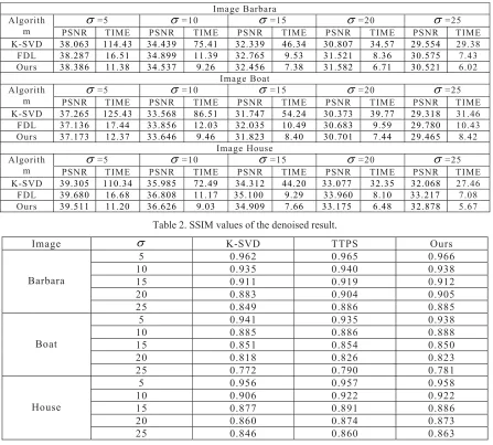
Table 1. PSNR values of the denoised results.

Image Barbara Algorith

m PSNR =5 TIME PSNR =10 TIME PSNR =15 TIME PSNR =20 TIME PSNR =25 TIME K-SVD 38.063 114.43 34.439 75.41 32.339 46.34 30.807 34.57 29.554 29.38 FDL 38.287 16.51 34.899 11.39 32.765 9.53 31.521 8.36 30.575 7.43 Ours 38.386 11.38 34.537 9.26 32.456 7.38 31.582 6.71 30.521 6.02

Image Boat Algorith

m PSNR =5 TIME PSNR=10 TIME PSNR=15 TIME PSNR=20 TIME PSNR=25 TIME K-SVD 37.265 125.43 33.568 86.51 31.747 54.24 30.373 39.77 29.318 31.46

FDL 37.136 17.44 33.856 12.03 32.035 10.49 30.683 9.59 29.780 10.43 Ours 37.173 12.37 33.646 9.46 31.823 8.40 30.701 7.44 29.465 8.42

Image House Algorith

[image:7.612.84.531.81.484.2]

m PSNR =5 TIME PSNR =10 TIME PSNR =15 TIME PSNR =20 TIME PSNR =25 TIME K-SVD 39.305 110.34 35.985 72.49 34.312 44.20 33.077 32.35 32.068 27.46 FDL 39.680 16.68 36.808 11.17 35.100 9.29 33.960 8.10 33.217 7.08 Ours 39.511 11.20 36.626 9.03 34.909 7.66 33.175 6.48 32.878 5.67

Table 2. SSIM values of the denoised result.

Image  K-SVD TTPS Ours

Barbara

5 0.962 0.965 0.966

10 0.935 0.940 0.938

15 0.911 0.919 0.912

20 0.883 0.904 0.905

25 0.849 0.886 0.885

Boat

5 0.941 0.935 0.938

10 0.885 0.886 0.888

15 0.851 0.854 0.850

20 0.818 0.826 0.823

25 0.772 0.790 0.781

House

5 0.956 0.957 0.958

10 0.906 0.922 0.922

15 0.877 0.891 0.886

20 0.860 0.874 0.873

[image:8.612.84.531.66.337.2]

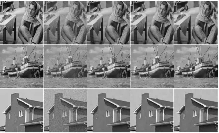
Figure 1. Displaying denoising results for, (a) original image (b) Noisy image, (c) Image denoised using K-SVDdictionary (d) Image denoised using FDL dictionary(e) Image denoised using Our dictionary. Table 1 presents the final denoising PSNR results obtained from K-SVD, FDL algorithms with additionally the fixed ours methods.The SSIM results of the three test methods are reported in Table 2. Figure displays the original, noisy and denoised “Barbara”, “Boat”, “House”, images for noise level =20. Based on these results, we can observe that our proposed algorithm, FTTSP algorithm, and FDL algorithm in general not only cost less time but also provide higher PSNR result and SSIM values in image denoising compared with the K-SVD algorithm. Although FTTSP algorithm and FDL algorithm have the similar results in general, it is noticeable that FTTSP algorithm needs less time compared with FDL.

Summary

In the paper, we present a fast top-bottom two-dimensional subspace partition algorithm (FTTSP algorithm) for learning overcomplete dictionary, which is based on a special partition tree structure. In construction of the partition tree step, our algorithm can obtain two level tree structures in every calculation, and hence it costs less time than the first part of the TTSP algorithm and FDL. It is equivalent to the second part of method SDL in construction dictionary step. Experimental results on synthetic data and imagepatches illustrate that FTTSP and FDL not only have higher quality but also cost less time than K-SVD, and that at the same time, FTTSP needs less time than FDL. In the future, we will consider improving FTTSP algorithm and applying it to other applications.

Acknowledgement

References

[1] D.L. Donoho, Compressed sensing, IEEE Trans on Information Theory. 52(4) (2006) 1289-1306. [2] M. Elad, M.A.T. Figueiredo and Y. Ma, On the role of sparse and redundant representations in image processing, Proceedings of the IEEE, 98 (6) (2010), 972–982.

[3] R. Tibshirani, Regression shrinkage and selection via the lasso, J. Royal. Statist. Soc B. 58(1) (2006) 267-288.

[4] S. Mallat and Z. Zhang, Matching pursuits with time-frequency dictionaries, IEEE Trans on Signal Proc. 41(12) (1993), 3397-3415.

[5] Y. Pati, R. Rezaiifar, P. Krishnaprasad, Orthogonal matching pursuit: Recursive function approximation with applications to wavelet decomposition, in Proceedings of the 27th Asilomar Conference on Signals, Systems & Computers. (1993) 40-44.

[6] S. Chen, D. Donoho, M. Saunders, Atomic decomposition by basis pursuit, SIAM Review. 43(1) (2001), 129-159.

[7] W. Dai, T. Xu, W. Wang, Simultaneous codeword optimization (SimCO) for dictionary update and learning, IEEE Trans on Signal Process. 60(12) (2012) 6341-6353.

[8] M. Elad, M. Aharon, Image denoising via sparse and redundant representations over learned dictionaries, IEEE Trans on Image Process. 15 (2006) 3736-3745.

[9] X. Zeng, W. Bian, W. Liu, J. Shen and D. Tao, Dictionary pair learning on Grassman manifolds for image denoising, IEEE Trans on Image Processing. 24 (11) (2015) 4556-4569.

[10] L. Liu, J. Ma, G. Plonka, Graph regularized seismic dictionary learning, http://num.math.uni- goettingen.de/plonka/pdfs/GraphDLrevised.pdf .

[11] X. Zeng, W. Bian, W. Liu, J. Shen and D. Tao, Dictionary pair learning on Grassman manifolds for image denoising, IEEE Trans on Image Processing. 24 (2015) 4556-4569.

[12] M. Zheng, J.J. Bu, C. Chen and C. Wang, Graph regularized sparse coding for image representation, IEEE Trans on Image Processing. 20(5) (2011), 920-930.

[13] T. Goldstein and S. Osher, The split Bregman method for L1-regularized problems, SIAM J. Imaging Sciences. 2(2) (2009) 323-343.

[14] G. Plonka and J. Ma, Curvelet-wavelet regularized split Bregman iteration for compressed sensing, Int. J. Wavelets Multiresolut Inf. Process. 9(1) (2011) 79-110.