http://dx.doi.org/10.4236/ojs.2016.64054
How to cite this paper: Doray, L.G., Luong, A. and Najem, E.-H. (2016) Efficiency of Some Estimators for a Generalized
Efficiency of Some Estimators for a
Generalized Poisson Autoregressive
Process of Order 1
Louis G. Doray
1, Andrew Luong
2, El-Halla Najem
11Département de Mathématiques et de Statistique, Université de Montréal, Montréal, Canada 2École d’Actuariat, Université Laval, Québec, Canada
Received 27 May 2016; accepted 20 August 2016; published 23 August 2016
Copyright © 2016 by authors and Scientific Research Publishing Inc.
This work is licensed under the Creative Commons Attribution International License (CC BY). http://creativecommons.org/licenses/by/4.0/
Abstract
Various models have been proposed in the literature to study non-negative integer-valued time series. In this paper, we study estimators for the generalized Poisson autoregressive process of
order 1, a model developed by Alzaid and Al-Osh [1]. We compare three estimation methods, the
methods of moments, quasi-likelihood and conditional maximum likelihood and study their asymptotic properties. To compare the bias of the estimators in small samples, we perform a si-mulation study for various parameter values. Using the theory of estimating equations, we obtain expressions for the variance-covariance matrices of those three estimators, and we compare their asymptotic efficiency. Finally, we apply the methods derived in the paper to a real time series.
Keywords
Discrete Time Series, Autoregressive Process, Moment Estimator, Quasi-Likelihood, Efficiency, Generalized Poisson, Quasi Binomial Distribution
1. Introduction
Time series are used to model various phenomena measured over time. Successive observations are often correlated, since they may depend on some common external factors, but which remain unknown to the analyst. In this case, autoregressive models will be useful to model this dependence.
( )
1PAR , introduced by Al-Osh and Alzaid [2] and the generalized Poisson autoregressive process of order 1, denoted GPAR
( )
1 (see Alzaid and Al-Osh [1]). The PAR( )
1 process, a stationary process with Poisson marginal distributions, is a special case of the GPAR( )
1 .The paper is organized as follows. In Section 2, for completeness, we review some properties of the generalized Poisson autoregressive process of order 1. In Section 3, we derive the expressions for the moments estimators, the quasi-likelihood and the maximum likelihood estimators of the 3 parameters of the GPAR
( )
1 . These methods have appeared in the literature (see Al-Nachawati, Alwasel and Alzaid [3] for the quasilike- lihood and moments method and Brännäs [4] for likelihood methods). However, asymptotic properties such as efficiencies of these methods are not discussed in those papers. In this paper (Sections 4 and 5), we study properties of these estimators such as bias and asymptotic efficiency. The last section reanalyzes a real-data example which can be modelled with a GPAR( )
1 process, where testing is discussed.We hope that with this study, practitioners will have more information to select one estimation method versus another one and to perform tests concerning values of the parameters.
2
GPAR
(1) Process
To define the GPAR
( )
1 process, we need first to review the generalized Poisson and the quasi-binomial distributions.A random variable X has a generalized Poisson distribution with parameters λ and θ, denoted GP
(
λ θ
,)
, if its probability mass function (pmf) is defined by[
]
(
)
1e( ) ! if 0,1, 2,...0 for , when 0,
x x
x x x
P X x
x m
λ θ
λ λ θ
θ
− − +
+ =
= =
> <
where λ>0, max
(
− −1,λ
m)
< ≤θ
1 and m( )
≥4 is the greatest positive integer for which λ+mθ>0 when θ is negative. Note that, for θ =0, the random variable X becomes a Poisson (λ) distribution. In this paper, we will restrict ourselves to the case where θ≥0.Consul [5] has shown that the expected value µ and variance σ2 of X
are given, when 0≤ <θ 1, by
(
)
2
3
and ,
1 1
λ
λ
µ
σ
θ
θ
= =
− −
so that, for positive values of θ, we have overdispersion (i.e. Var
[ ]
X >E X[ ]
).The sum X+Y of two independent random variables X and Y with GP
(
λ θ
1,)
and GP(
λ θ
2,)
distributions, also has a GP distribution, with parameters
(
λ λ θ
1+ 2,)
. Ambagaspitiya and Balakrishnan [6]have derived the recurrence formula for the probability function of the compound generalized Poisson distribution, used in risk theory.
A non-negative integer-valued random variable X has a quasi-binomial distribution, denoted QB p
(
, ,θ
n)
, if its pmf is given by[
]
(
)
(
)
(
)
1 1
1 , 0,1, 2, , ,
1
n x x
n n
pq p x q n x
x
P X x x n
n
θ θ
θ
− − −
−
+ + −
= = =
+
where 0< <p 1,q= −1 p and θ is such that n
θ
<min(
p q,)
. Its mean, equal to pn, is independent of the parameter θ.The following proposition, proved in Alzaid and Al-Osh [1], shows the relation between the QB and GP distributions.
Proposition 1: If X and S n
( )
are two independent random variables with GP(
λ θ
,)
and QB p(
,θ λ
,n)
distributions, then S X
( )
follows a GP p(
λ θ
,)
distribution.The GPAR
( )
1 process generalizes the PAR( )
1 process introduced by Al-Osh and Alzaid [2]. The( )
1PAR model, where Var
[ ]
Xt =E X[ ]
t , has been used to model time series in various fields, for example in insurance for short-term workers' compensation because of work-related injuries (Freeland and McCabe [7]) and in medicine for the incidence of infectious diseases (Cardinal, Roy and Lambert [8]).[ ]
tE X ). The PAR
( )
1 model would therefore not be appropriate for those time series. In cases where the extra variation can be explained in a deterministic way, adding regressors would be adequate (see Freeland and McCabe [7]), but where the extra variation is of a stochastic nature, the GPAR( )
1 model could be used for modelling overdispersed time series.The GPAR
( )
1 model, introduced by Alzaid and Al-Osh [1], is defined as(
1)
, 1, 2,t t t t
X =S X− +
ε
t= (1)where
1)
{
St( )
• ,t=1, 2,}
is a sequence of iid random variables with a QB p(
,θ λ
,•)
distribution. 2){ }
ε
t is a sequence of iid random variables with a GP q(
λ θ
,)
distribution.3) These two sequences are independent of each other.
4) X0 has a GP
(
λ θ
,)
distribution independent of{ }
ε
t and{
St( )
•}
.Proposition 2: The GPAR
( )
1 process{ }
Xt has a GP marginal distribution.Proof: See Alzaid and Al-Osh [1]. The GPAR
( )
1 process is obtained from the QB p(
,θ λ
,•)
and(
,)
GP q
λ θ
distributions, and not from the QB p(
, ,θ
•)
and GP q(
λ θ
,)
distributions, as stated in Al- Nachawati et al. [3].The autocorrelation function (acf) of the GPAR
( )
1 process{ }
Xt is equal to( )
Corr[
,]
k, for 0,1, 2, .X k X Xt t k p k
ρ = − = =
The acf of this process is the same as that of an AR
( )
1 process except that it is always non-negative, since( )
0,1p∈ . The partial autocorrelation function (pacf) of the GPAR
( )
1 process is equal to if 10 if 2, 3,
kk
p k
k
φ
= ==
The sample acf and pacf will be useful to identify the GPAR
( )
1 model from an observed time series.3. Estimation of the Parameters
Estimating the parameters in a GPAR
( )
1 process will present some challenges, since the conditional distribution of Xt, given Xt−1=xt−1, is the convolution of a QB p(
,θ λ
,xt−1)
and a GP q(
λ θ
,)
distri-bution.
In this section, we will review three estimation methods for the parameter vector Θ =
(
p, ,λ θ
)
of the( )
1GPAR process, the methods of moments, quasi-likelihood and conditional maximum likelihood. These methods have been proposed in the literature, see for example, Al-Nachawati et al. [3] or Brännäs [4]. However, less emphasis is placed on their asymptotic properties, such as efficiency. In Section 4, we study the bias of these estimators, and in Section 5 their efficiency.
3.1. Method of Moments or Yule-Walker
The first autocovariance of the GPAR
( )
1 process is equal to[
1]
[ ]
0Cov Xt+,Xt = pVar X . (2) By taking the expected value of both sides of the equation given in (1), we find
[ ]
(
1)
.t
t t
E X =E S X − +µε Since
(
t1)
Xt1{
(
t1)
| t1 t1}
[
t1]
, E S X − =E − E S X − X− =x− =E pX−we obtain
[ ]
[
1]
. 1t t
q
E X pE X λ
θ
−
= +
− (3) We also know that
[ ]
(
)
3Var .
1
t
X
λ
θ
=
− (4)
From the observations x x1, 2,,xn, we estimate the means E X
[ ]
t , E X[ ]
t−1 , the variance Var[ ]
Xt and1 1 , n t t x x n = =
∑
1 0 1 1 , 1 n t t x x n − = = −∑
[ ]
(
)
21 1 Var , n t t t
X x x
n =
=
∑
−[
]
1(
)(
)
1 1
1
1
Cov , .
n
t t t t
t
X X x x x x
n
−
+ +
=
=
∑
− −Solving the system of Equations (2), (3), (4) with E X
[ ]
t , E X[ ]
t−1 , Var[ ]
Xt and Cov[
Xt+1,Xt]
replaced by their sample values, we obtain the moments estimators Θ =(
p, ,λ θ)
of parameter vector Θ =(
p, ,λ θ
)
,(
)(
)
(
)
1 1 1 2 1 n t t t n t tx x x x
p x x − + = = − − = −
∑
∑
(
)
(
)
3 0 2 3 1 n t t n x pxq x x
λ = − = −
∑
(
0)
1 q
x px
λ
θ
= −−
where q= −1 p.
We have corrected here misprints in the formulas for the moment estimators of the parameters λ and θ given by Al-Nachawati et al. [3].
3.2. Quasi-Likelihood Method
This method, proposed initially by Whittle [9], replaces the true likelihood by the one which assumes that the observations come from a normal distribution with the same conditional mean and variance. Al-Nachawati et al. [3] obtained the quasi-likelihood estimators Θ =
(
p, ,λ θ )
by maximizing(
)
( )2 2 22 1
1
, , e
2π
t t t
n
x
t
t
L pλ θ µ σ
σ
− −
= =
∏
where µt and
σ
t2 are given by[
]
( )
(
)
1 1 1 1 | 1 , tt t t t
t t
E X X x
E S x
px q ε µ µ λ θ − − − − = = = + = + − and
[
]
(
)
[ ]
(
)
(
)
(
)
(
)
1 2 1 11 1 1
1 1 3 1 2 1 1 1 1 Var |
Var | Var
!
1 .
1 ! 1
t
t t t t
t t t t t
j x t t j j t t
X X x
S X X x
x
pq x q
x j x
σ
ε
θ λ λ θ
θ λ − − − − − − − − − − = − − = = = = + = − + − − − +
∑
which is a bit different from the one given in Al-Nachawati et al. [3]. Since the GPAR
( )
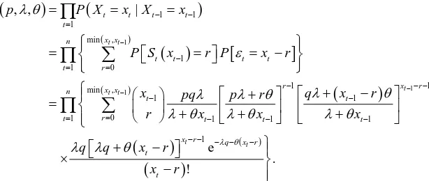
1 process is restricted to non-negative integers and therefore not symmetrical, one might suspect that the estimators are less efficient than the maximum likelihood estimators, which is indeed the case (see Section 5 for numerical results).3.3. Conditional Maximum Likelihood Method
To obtain the conditional maximum likelihood estimators (MLE’s) Θ =ˆ
(
pˆ , ,λ θˆ ˆ)
, we need the conditional distribution of(
Xt |Xt−1=xt−1)
, which is the convolution of a QB p(
,θ λ
,xt−1)
distribution and a(
,)
GP q
λ θ
distribution. Given the observations x x x0, 1, 2,,xn, we have to maximize the function(
)
(
)
( )( )
[
]
( )(
)
(
)
1 1 1 1 1 1 min , 1 0 1 1 1 min , 1 1 01 1 1 1
1 , , | e t t t t t t n
t t t t
t
x x n
t t t t
r t x r r x x n t t r
t t t t
x r t
L p P X x X x
P S x r P x r
x pq p r q x r
r x x x
q q x r
λ θ
ε
λ θ
λ λ θ
λ θ λ θ λ θ
λ λ θ
− − − − − = − = = − − − − − = = − − − − − − = = = = = = − + + − = + + + + − ×
∏
∑
∏
∑
∏
( )(
)
! . tq x r
t
x r
λ θ− −
−
We will work with the loglikelihood function l p
(
, ,λ θ
)
, equal to lnL p(
, ,λ θ
)
, which will have to be maximized numerically to obtain the MLE Θˆ.Under normal regularity conditions, using likelihood theory (see Gouriéroux and Monfort [11] or Hamilton [12]), the vector Θˆ has an asymptotic multinormal distribution, i.e.
(
ˆ)
(
1( )
)
0, ,
n Θ − Θ →N I− Θ
where → denotes convergence in law, 0 is the vector of zeros of dimension 3, and
( )
2( )
i j
I E l
θ θ
∂ Θ = − ∂ ∂ Θ
is Fisher’s expected information matrix, of dimension 3 3
× .
4. Bias of Estimators
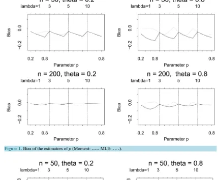
With simulations, we will study the bias of the moments estimators and the MLE’s. Setting the values of the 3 parameters to those in Table 1, two series of 50 and 200 observations were generated from model (1) in C++. This experiment was repeated 200 times.
For each series, the moments estimators were calculated, as well as their average, and the bias. The conditional MLE's were calculated using the iterative Downhill Simplex method (see Press, Teukolsky, Vetterling and Flannery [13]), which does not require the calculation of the derivatives of the function to be maximized. As initial values, we used the moments estimators. The results of the simulations appear in Figures 1-3.
[image:5.595.162.469.197.327.2]From Figures 1-3, we see that the bias of the MLE’s is smaller than that of the moments estimators, and that
Table 1. Values of parameters.
p λ θ
0.2 1 0.2
0.4 3 0.4
0.6 5 0.6
Figure 1. Bias of the estimators of p (Moment: --- MLE: - - -).
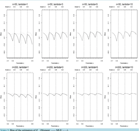
Figure 3. Bias of the estimators of θ (Moment: --- MLE: - - -).
it decreases when the size of the series increases. Figure 1 shows that the bias of pˆ is much smaller than that of p, except when n=200 and θ =0.2 where they are almost equal to 0. The bias of the two estimators is negative. In Figure 2, we see that the bias of λˆ and
λ
is close to 0 when λ=1; as λ increases, λˆ andλ
are more biased. In all cases, the bias of the estimator of λ is positive. The bias of the estimator of θ behaves like that of p (Figure 3); for the two estimation methods, it is similar for λ=5 or 10.Since the moments estimators and the conditional MLE’s are almost unbiased for large n, we study their asymptotic efficiency in the next section.
5. Asymptotic Efficiency of Estimators
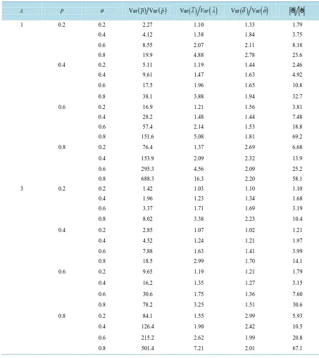
Table 2. Efficiency of moments estimators.
λ p θ Var
( )
p Var( )
pˆ Var( )
λ Var( )
λˆ Var( )
θ Var( )
θˆ Θ Θˆ1 0.2 0.2 2.27 1.10 1.33 1.79
0.4 4.12 1.38 1.84 3.75
0.6 8.55 2.07 2.11 8.18
0.8 19.9 4.88 2.78 23.6
0.4 0.2 5.11 1.19 1.44 2.46
0.4 9.61 1.47 1.63 4.92
0.6 17.5 1.96 1.65 10.8
0.8 38.1 3.88 1.94 32.7
0.6 0.2 16.9 1.21 1.56 3.81
0.4 28.2 1.48 1.44 7.48
0.6 57.4 2.14 1.53 18.8
0.8 151.6 5.08 1.81 69.2
0.8 0.2 76.4 1.37 2.69 6.68
0.4 153.9 2.09 2.32 13.9
0.6 295.3 4.56 2.09 25.2
0.8 688.3 16.3 2.20 58.1
3 0.2 0.2 1.42 1.03 1.10 1.10
0.4 1.96 1.23 1.34 1.68
0.6 3.37 1.71 1.69 3.19
0.8 8.02 3.38 2.23 10.4
0.4 0.2 2.85 1.07 1.02 1.21
0.4 4.52 1.24 1.21 1.97
0.6 7.88 1.63 1.41 3.99
0.8 18.5 2.99 1.70 14.1
0.6 0.2 9.65 1.19 1.21 1.79
0.4 16.2 1.35 1.27 3.15
0.6 30.6 1.75 1.36 7.60
0.8 78.2 3.25 1.51 30.6
0.8 0.2 84.1 1.55 2.99 5.93
0.4 126.4 1.90 2.42 10.5
0.6 215.2 2.62 1.99 20.8
0.8 501.4 7.21 2.01 67.1
5.1. Method of Moments
By using an asymptotically equivalent factor of 1n instead of 1n−1 in Equation (3), moments estimators
(
p, ,λ θ)
Θ = are given as solutions of the system of equations
(
)
(
)(
)
(
)
1
1 2 1
1
1
0
n
t t
n t
t t
n X X X X
p
X X
− +
=
=
− − −
− =
−
∑
Table 3. Efficiency of quasi-likelihood estimators.
λ p θ Var
( )
p Var( )
pˆ Var( )
λ Var( )
λˆ Var( )
θ Var( )
θˆ Θ Θ ˆ1 0.2 0.2 2.06 1.07 1.18 2.25
0.4 3.16 1.25 1.73 5.09
0.6 7.17 2.30 1.82 15.3
0.8 12.4 7.39 2.48 48.5
0.4 0.2 2.03 1.08 1.35 2.49
0.4 3.07 1.36 1.67 5.14
0.6 5.79 2.73 1.99 15.9
0.8 14.7 15.4 3.22 98.4
0.6 0.2 1.94 1.30 1.66 3.63
0.4 2.46 1.46 1.97 5.95
0.6 5.91 4.08 2.83 23.0
0.8 30.6 19.8 5.62 38.2
0.8 0.2 2.27 2.14 2.94 12.0
0.4 4.03 2.94 4.45 19.0
0.6 14.8 13.7 6.61 90.6
0.8 120.1 44.4 16.1 41.9
3 0.2 0.2 1.37 1.03 1.09 1.40
0.4 1.79 1.16 1.25 2.12
0.6 2.72 1.52 1.50 4.24
0.8 6.23 3.04 1.94 17.6
0.4 0.2 1.39 1.08 1.12 1.37
0.4 1.82 1.19 1.23 2.12
0.6 2.72 1.58 1.52 4.55
0.8 5.47 3.29 2.03 17.5
0.6 0.2 1.76 1.27 1.41 1.88
0.4 2.32 1.44 1.49 3.21
0.6 3.01 1.87 1.82 6.87
0.8 6.36 4.15 2.69 26.0
0.8 0.2 3.67 1.88 3.01 6.50
0.4 3.92 2.19 2.52 12.6
0.6 6.61 2.94 2.97 32.4
0.8 12.0 8.34 5.39 58.5
(
) (
)
1
1
1 0
1 n
t t
p
X p λ
θ
=
−
− − =
−
∑
(
)
2(
)
3 1
0. 1
n t t
X X λ
θ
=
− − =
−
∑
Let us define the functions
(
) (
)
(
)(
)
(
)
1 2 1
1
, , t t
t n
t t
n X X X X
f p p
X X
λ θ +
=
− − −
= −
−
(
, ,)
(
1) (
1)
1t t
p
g pλ θ X p λ
θ
−
= − −
−
(
)
(
)
2(
)
3
, ,
1
t t
h p
λ θ
X Xλ
θ
= − −
−
and the vector
( )
1(
)
(
)
(
)
1 1 1
, , , , , , , , .
n n n
n t t t
t t t
F f p
λ θ
g pλ θ
h pλ θ
−
= = =
Θ =
∑
∑
∑
The expected values E f t
(
p, ,λ θ)
, E g t(
p, ,λ θ)
and E h p t(
, ,λ θ)
are asymptotically equal to 0. Using a Taylor series expansion around Θ =0(
p0,λ θ
0, 0)
, the true parameter value, we obtain( )
( )
0( )
0(
0)
,n n n
F Θ =F Θ + ∇F Θ Θ − Θ +ε (5)
where p 0
nε → , with →p denoting convergence in probability.
Since Θ is a solution of Fn
( )
Θ =0, Equation (5) can rewritten as( )
0(
0)
( )
0 ,n n
F F ε
∇ Θ Θ − Θ = − Θ −
or 1 Fn
( )
0 n(
0)
1Fn( )
0 op( )
1 .n n
−
∇ Θ Θ − Θ = Θ +
Using Slutsky’s theorem, we find that
( )
0(
0)
( )
01 1
,
n n
F n F
n∇ Θ Θ − Θ → n Θ
or n
(
0)
N 0,A1Var( )
Y( )
A1 ,− −
′
Θ − Θ → (6) where, with probability 1,
( )
( )
01 1
lim n and lim n .
n n
A F Y F
n n
→∞ →∞
= ∇ Θ = − Θ
Matrix A evaluated at Θ0 can be estimated by
(
)
(
)
(
)
(
)
(
)
0 0 0
0
2
0 0 0
0
3 4
0 0
1 0 0
1 1
1
ˆ .
1 1 1
3 0
1 1
n
n p n p
n A nx n n n λ λ
θ θ θ
λ θ θ − + − − = − + − − − − − − − − −
If θ λ0, 0 and p0 are unknown, they can be replaced by appropriate estimates. The variance-covariance matrix of Y is equal to
(
)
(
)
(
)
(
)
(
)
(
)
(
)
(
)
(
)
1 1 1 1 1
1 1 1 1 1
1 1 1 1 1
Var Cov , Cov ,
1
Cov , Var Cov , .
Cov , Cov , Var
n n n n n
t t t t t
i i i i i
n n n n n
t t t t t
i i i i i
n n n n n
t t t t t
i i i i i
f f g f h
g f g g h
n
h f h g h
= = = = = = = = = = = = = = =
∑
∑
∑
∑
∑
∑
∑
∑
∑
∑
∑
∑
∑
∑
∑
Let us consider the first element of this matrix:
[
]
1 1 1
=1 1 1
1 1
Var ,
n n n
t t k
t t k
f E f f
since asymptotically E f f
[
t k]
=Cov(
f ft, k)
(because E f[ ]
t =0 as n→ ∞). In practice, we truncate theseexpressions, since Cov
(
f ft, k)
→0, as t− → ∞k . If we limit ourselves to a difference of t− ≤k 5, the last equality becomes[
]
1
=1 5
1 1
Var ) .
n
t t k
t t k
f E f f
n n − − ≤
∑
∑ ∑
Using the law of large numbers, we can estimate this last term by
5 1 . t k t k f f n
∑ ∑
− ≤The other elements of the matrix can be estimated in the same way.
5.2. Quasi-Likelihood Method
To determine the quasi-likelihood estimator
( )
Θ , we have to maximize(
)
( )
( )
2(
)
22 1
, , 0.5 ln 2π 0.5 ln .
n
t t t
t t
x
l p λ θ n σ µ
σ = − = − − +
∑
(7)Let us define the quasi-score vector
( )
( )
(
( )1 ( )2 ( )3)
( )
( )
( )
, , , , .
t t t t
S l S S S l l l
p λ θ
′
∂ ∂ ∂
′
Θ = ∇ Θ = = Θ Θ Θ
∂ ∂ ∂
From Hamilton [12], using quasi-likelihood theory, we conclude that
(
)
(
1 1)
0 0, ,
n Θ − Θ ′→ N D SD− − (8) where with probability 1, D and S are limits in probability matrices. They are defined as
( )
(
)
(
( ))
(
( ))
( )(
)
(
( ))
(
( ))
( )(
)
(
( ))
1 1 1
1 1 1
1 1 1
2 2 2
1 1 1
1 1 1
3 3
1 1
1 1 1
| | |
1
lim | | |
| |
n n n
t t t t t t
t t t
n n n
t t t t t t
t t t
n
n n n
t t t t
t t t
E S X E S X E S X
p
D E S X E S X E S X
n p
E S X E S X
p λ θ λ θ λ − − − = = = − − − = = = →∞ − − = = = ∂ ∂ ∂ ∂ ∂ ∂ ∂ ∂ ∂ = − ∂ ∂ ∂ ∂ ∂ ∂ ∂
∑
∑
∑
∑
∑
∑
∑
∑
∑
(
( )3)
1
,
|
t t
E S X
θ − ∂ ∂ and ( ) ( ) ( ) ( ) ( ) ( ) ( ) ( ) ( ) ( ) ( ) ( ) ( ) ( ) ( ) ( ) ( ) ( )
1 1 1 2 1 3
1 1 1
2 1 2 2 2 3
1 1 1
3 1 3 2 3 3
1 1 1
1
lim ,
n n n
t t t t t t
t t t
n n n
t t t t t t
t t t
n
n n n
t t t t t t
t t t
S S S S S S
S S S S S S S
n
S S S S S S
= = = = = = →∞ = = = =
∑
∑
∑
∑
∑
∑
∑
∑
∑
evaluated at Θ0, the true parameter. We can obtain estimates for Dˆ and Sˆ, where matrix Dˆ is defined as
( )
(
)
(
( ))
(
( ))
( )(
)
(
( ))
(
( ))
( )(
)
(
( ))
(
( ))
1 1 1
1 1 1
1 1 1
2 2 2
1 1 1
1 1 1
3 3 3
1 1 1
1 1 1
| | |
1
ˆ | | | ,
| | |
n n n
t t t t t t
t t t
n n n
t t t t t t
t t t
n n n
t t t t t t
t t t
S X S X S X
p
D S X S X S X
n p
S X S X S X
p λ θ λ θ λ θ − − − = = = − − − = = = − − − = = = ∂ ∂ ∂ ∂ ∂ ∂ ∂ ∂ ∂ = − ∂ ∂ ∂ ∂ ∂ ∂ ∂ ∂ ∂
∑
∑
∑
∑
∑
∑
∑
∑
∑
expression (7). Packages such as MATHEMATICA can handle these derivatives calculations numerically. Consequently, the variance-covariance matrix of Θ can be estimated by D SDˆ−1ˆˆ−1.
5.3. Conditional Maximum Likelihood
Using the true loglikelihood function from section 4.3, we define the score vector
( )
( )
(
( )1 ( )2 ( )3)
, , .
t t t t
S Θ = ∇ Θ =l S S S ′
From Hamilton [12], using likelihood theory, we find that
(
)
(
1)
0
ˆ 0, ,
n Θ − Θ →N S− (9)
where matrix S is defined analogously as in the previous section, but with a different loglikelihood function.
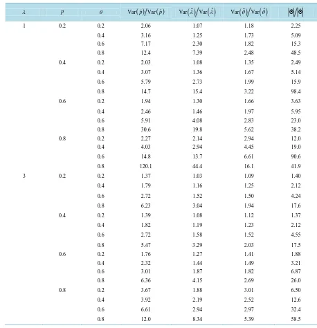
5.4. Numerical Comparisons
Table 2 and Table 4 give the estimate of the asymptotic efficiency of the moment and the quasi-likelihood estimators compared to the MLE, calculated from 20,000 observations (10 series of 2000 observations) gene- rated from a GPAR
( )
1 process with various parameter values.Comparing Table 2 and Table 3, the quasi-likelihood estimator for p has a smaller variance than the moments estimator; for λ, it depends on the values of the parameters. The moments estimator of θ has a smaller variance than the quasi-likelihood estimator, except when p=0.2, where θ is better than
θ
.The estimated determinant of the variance-covariance matrix of Θˆ using the average of the determinants is always smaller than that of Θ and Θ (last column of Table 2 and Table 3). The MLE is more efficient than the moment or the quasi-likelihood estimator, and the moment estimator more efficient than the quasi-likelihood estimator, in general.
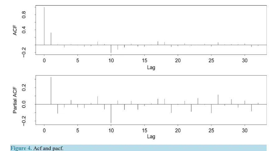
6. Applications: Number of Computer Breakdowns
In this section, we perform some tests on a real time series presented by Al-Nachawati et al. [3] on the number of weekly computer breakdowns for 128 consecutive weeks. This series is overdispersed, since its mean and variance are equal to 4.016 and 14.504. In Figure 4, the acf function is seen to decrease with the lag, while the pacf is high for lag 1 and low thereafter; a GPAR
( )
1 model could therefore be appropriate for this series. We use the GPAR( )
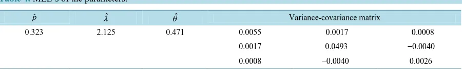
1 model in the analysis.Since the MLE was shown to be the best asymptotic estimator in the previous section, the parameters were estimated with this method; the estimates appear in Table 4, with the estimated variance-covariance matrix.
With the estimated variance-covariance matrices based on expressions (6), (8) and (9) of Section 5, Wald tests can be performed quite easily depending on which estimator has been chosen.
For example, to test H0:θ θ= 0 using θ, the quasilikelihood estimator, the statistic can be based on the statistic Z =
(
θ θ− 0)
V( )
θ , where V( )
θ is an estimate of the variance of θ, which can be obtained from the corresponding diagonal element of Vˆ=D SDˆ−1ˆˆ−1. Since(
θ θ− 0)
V( )
θ is asymptotically N( )
0,1 , we reject H0 at level α if Z is greater than z1−α2.To test H0:p= p0,λ λ θ θ= 0, = 0, the test statistic can be based on
1
0 Vˆ 0 ,
− ′
Θ − Θ Θ − Θ
[image:12.595.88.538.650.719.2]which follows a χ2
( )
3 distribution asymptotically. It is expected that the more efficient the estimator is, theTable 4. MLE’s of the parameters.
ˆ
p λˆ θˆ Variance-covariance matrix
0.323 2.125 0.471 0.0055 0.0017 0.0008
0.0017 0.0493 −0.0040
Figure 4. Acf and pacf.
more powerful the test will be.
With the estimated parameters, we can test the GPAR
( )
1 model versus the simpler PAR( )
1 model. Since the conditional MLE θˆ equals 0.471, with a variance of 0.0026, performing the test H0:θ =0 vs H1:θ >0 gives Z =0.471 0.0026=9.24. This leads us to reject H0 and to conclude that the GPAR( )
1 model is more appropriate: there is overdispersion in the observations.Acknowledgements
The authors gratefully acknowledge the financial support of the Natural Sciences and Engineering Research Council of Canada and of the Fonds pour la Contribution à la Recherche du Québec.
References
[1] Alzaid, A.A. and Al-Osh, M.A. (1993) Some Autoregressive Moving Average Processes with Generalized Poisson Marginal Distributions. Annals of the Institute of Mathematical Statistics, 45, 223-232.
http://dx.doi.org/10.1007/BF00775809
[2] Al-Osh, M.A. and Alzaid, A.A. (1987) First-Order Integer-Valued Autoregressive (INAR(1)) Process. Journal of Time Series Analysis, 8, 261-275. http://dx.doi.org/10.1111/j.1467-9892.1987.tb00438.x
[3] Al-Nachawati, H., Alwasel, I. and Alzaid, A.A. (1997) Estimating the Parameters of the Generalized Poisson AR(1) process. Journal of Statistical Computation and Simulation, 56, 337-352.
http://dx.doi.org/10.1080/00949659708811798
[4] Brännäs, K. (1994) Estimation and Testing in Integer-Valued AR(1) Models. Umeå Economic Studies 335, Umeå, Sweden.
[5] Consul, P.C. (1989) Generalized Poisson Distribution: Properties and Applications. Marcel Dekker Inc., New York. [6] Ambagaspitiya, R.S. and Balakrishnan, N. (1994) On the Compound Generalized Poisson Distributions. ASTIN
Bulle-tin, 24, 255-263. http://dx.doi.org/10.2143/AST.24.2.2005069
[7] Freeland, R.K. and McCabe, B. (2004) Analysis of Low Count Time Series Data by Poisson Autoregression. Journal of Time Series Analysis, 25, 701-722. http://dx.doi.org/10.1111/j.1467-9892.2004.01885.x
[8] Cardinal, M., Roy, R. and Lambert, J. (1999) On the Application of Integer-Valued Time Series Models for the Analy-sis of Disease Incidence. Statistics in Medicine, 18, 2025-2039.
http://dx.doi.org/10.1002/(SICI)1097-0258(19990815)18:15<2025::AID-SIM163>3.0.CO;2-D
[9] Whittle, P. (1961) Gaussian Estimation in Time Series. Bulletin of the International Statistical Institute, 39, 1-26. [10] Shenton, L.R. (1986) Quasi-Binomial Distributions. Encyclopedia of Statistical Sciences, John Wiley & Sons, New
[11] Gouriéroux, C. and Monfort. A. (1983) Cours de Hamilton, J.D. (1994) Time Series Analysis. Princeton University Press, New Jersey.
[12] Hamilton, J.D. (1994) Time Series Analysis. Princeton University Press, New Jersey.
[13] Press, W.H., Teukolsky, S.A., Vetterling, W.T. and Flannery, B.P. (2002) Numerical Recipies in C++. The Art of Scientific Computing. Cambridge University Press, Cambridge.
Submit or recommend next manuscript to SCIRP and we will provide best service for you:
Accepting pre-submission inquiries through Email, Facebook, LinkedIn, Twitter, etc. A wide selection of journals (inclusive of 9 subjects, more than 200 journals) Providing 24-hour high-quality service
User-friendly online submission system Fair and swift peer-review system
Efficient typesetting and proofreading procedure
Display of the result of downloads and visits, as well as the number of cited articles Maximum dissemination of your research work