Munich Personal RePEc Archive
Estimating structural VARMA models
with uncorrelated but non-independent
error terms
Boubacar Mainassara, Yacouba and Francq, Christian
Université Lille III, EQUIPPE-GREMARS, Université Lille III,
EQUIPPE-GREMARS
2009
Estimating structural VARMA models with
uncorrelated but non-independent error terms
Y. Boubacar Mainassaraa
, C. Francqb
a
Université Lille III, EQUIPPE-GREMARS, BP 60 149, 59653 Villeneuve d’Ascq cedex, France.
b
Université Lille III, EQUIPPE-GREMARS, BP 60 149, 59653 Villeneuve d’Ascq cedex, France.
Abstract
The asymptotic properties of the quasi-maximum likelihood estimator (QMLE) of vector autoregressive moving-average (VARMA) models are de-rived under the assumption that the errors are uncorrelated but not nec-essarily independent. Relaxing the independence assumption considerably extends the range of application of the VARMA models, and allows to cover linear representations of general nonlinear processes. Conditions are given for the consistency and asymptotic normality of the QMLE. A particular attention is given to the estimation of the asymptotic variance matrix, which may be very different from that obtained in the standard framework. Modi-fied versions of the Wald, Lagrange Multiplier and Likelihood Ratio tests are proposed for testing linear restrictions on the parameters.
Key words: Echelon form, Lagrange Multiplier test, Likelihood Ratio test, Nonlinear processes, QMLE, Structural representation, VARMA models, Wald test.
1. Introduction
This paper is devoted to the problem of estimating VARMA representa-tions of multivariate (nonlinear) processes.
Email addresses: mailto:[email protected](Y. Boubacar Mainassara),[email protected](C. Francq)
In order to give a precise definition of a linear model and of a nonlinear process, first recall that by the Wold decomposition (see e.g. Brockwell and Davis, 1991, for the univariate case, and Reinsel, 1997, in the multivariate framework) any zero-mean purely non deterministicd-dimensional stationary process (Xt) can be written in the form
Xt= ∞
X
ℓ=0
Ψℓǫt−ℓ, (ǫt)∼WN(0,Σ) (1)
whereP
ℓkΨℓk2 <∞. The process(ǫt)is called the linear innovation process
of the process X = (Xt), and the notation(ǫt)∼WN(0,Σ) signifies that(ǫt)
is a weak white noise. A weak white noise is a stationary sequence of cen-tered and uncorrelated random variables with common variance matrix Σ. By contrast, a strong white noise, denoted by IID(0,Σ), is an independent and identically distributed (iid) sequence of random variables with mean 0 and varianceΣ. A strong white noise is obviously a weak white noise, because independence entails uncorrelatedness, but the reverse is not true. Between weak and strong white noises, one can define a semi-strong white noise as a stationary martingale difference. An example of semi-strong white noise is the generalized autoregressive conditional heteroscedastic (GARCH) model. In the present paper, a process X is said to be linear when (ǫt)∼IID(0,Σ)
in (1), and is said to be nonlinear in the opposite case. With this definition, GARCH-type processes are considered as nonlinear. Leading examples of linear processes are the VARMA and the sub-class of the vector autoregres-sive (VAR) models with iid noise. Nonlinear models are becoming more and more employed because numerous real time series exhibit nonlinear dynam-ics, for instance conditional heteroscedasticity, which can not be generated by autoregressive moving-average (ARMA) models with iid noises.1
The main issue with nonlinear models is that they are generally hard to identify and implement. This is why it is interesting to consider weak (V)ARMA models, that is ARMA models with weak white noises, such linear
1To cite few examples of nonlinear processes, let us mention the self-exciting threshold
representations being universal approximations of the Wold decomposition (1). Linear and nonlinear processes also have exact weak ARMA representa-tions because a same process may satisfy several models, and many important classes of nonlinear processes admit weak ARMA representations (see Francq, Roy and Zakoïan, 2005, and the references therein).
The estimation of autoregressive moving-average (ARMA) models is how-ever much more difficult in the multivariate than in univariate case. A first difficulty is that non trivial constraints on the parameters must be imposed for identifiability of the parameters (see Reinsel, 1997, Lütkepohl, 2005). Sec-ondly, the implementation of standard estimation methods (for instance the Gaussian quasi-maximum likelihood estimation) is not obvious because this requires a constrained high-dimensional optimization (see Lütkepohl, 2005, for a general reference and Kascha, 2007, for a numerical comparison of alter-native estimation methods of VARMA models). These technical difficulties certainly explain why VAR models are much more used than VARMA in applied works. This is also the reason why the asymptotic theory of weak ARMA model estimation is mainly limited to the univariate framework (see Francq and Zakoïan, 2005, for a review on weak ARMA models). Notable exceptions are Dufour and Pelletier (2005) who study the asymptotic prop-erties of a generalization of the regression-based estimation method proposed by Hannan and Rissanen (1982) under weak assumptions on the innovation process, and Francq and Raïssi (2007) who study portmanteau tests for weak VAR models.
For the estimation of ARMA and VARMA models, the commonly used estimation method is the QMLE, which can also be viewed as a nonlinear least squares estimation (LSE). The asymptotic properties of the QMLE of VARMA models are well-known under the restrictive assumption that the errors ǫt are independent (see Lütkepohl, 2005). The asymptotic behavior
able to cover weak VARMA representations of general nonlinear models. The paper is organized as follows. Section 2 presents the structural weak VARMA models that we consider here. Structural forms are employed in econometrics in order to introduce instantaneous relationships between eco-nomic variables. The identifiability issues are discussed. It is shown in Sec-tion 3 that the QMLE is strongly consistent when the weak white noise(ǫt)is
ergodic, and that the QMLE is asymptotically normally distributed when(ǫt)
satisfies mild mixing assumptions. The asymptotic variance of the QMLE may be very different in the weak and strong cases. Section 4 is devoted to the estimation of this covariance matrix. In Section 5 it is shown how the standard Wald, LM (Lagrange multiplier) and LR (likelihood ratio) tests must be adapted in the weak VARMA case in order to test for general linear-ity constraints. This section is also of interest in the univariate framework because, to our knowledge, these tests have not been studied for weak ARMA models. Numerical experiments are presented in Section 6. The proofs of the main results are collected in the appendix.
2. Model and assumptions
Consider a d-dimensional stationary process (Xt) satisfying a structural VARMA(p, q)representation of the form
A00Xt− p
X
i=1
A0iXt−i =B00ǫt− q
X
i=1
B0iǫt−i, (ǫt)∼WN(0,Σ0), (2)
where Σ0 is non singular and t ∈ Z = {0,±1, . . .}. The standard
VARMA(p, q)form, which is sometimes called the reduced form, is obtained for A00 = B00 = Id. The structural forms are mainly used in econometrics
to identify structural economic shocks and to allow instantaneous relation-ships between economic variables. Of course, constraints are necessary for the identifiability of the (p+q+ 3)d2 elements of the matrices involved in
the VARMA equation (2). We thus assume that these matrices are param-eterized by a vector ϑ0 of lower dimension. We then write A0i = Ai(ϑ0)
and B0j = Bj(ϑ0) for i = 0, . . . , p and j = 0, . . . , q, and Σ0 = Σ(ϑ0), where
ϑ0 belongs to the parameter space Θ ⊂ Rk0, and k0 is the number of
un-known parameters, which is typically much smaller that (p+q+ 3)d2. The
A1: The applications ϑ 7→ Ai(ϑ) i = 0, . . . , p, ϑ 7→ Bj(ϑ) j = 0, . . . , q
and ϑ 7→Σ(ϑ) admit continuous third order derivatives for all ϑ∈Θ.
For simplicity we now write Ai, Bj and Σ instead of Ai(ϑ), Bj(ϑ) and Σ(ϑ). LetAϑ(z) =A0−Ppi=1Aizi andBϑ(z) =B0−Pqi=1Bizi. We assume
that Θ corresponds to stable and invertible representations, namely
A2: for all ϑ∈Θ, we have detAϑ(z) detBϑ(z)6= 0 for all |z| ≤1.
To show the strong consistency of the QMLE, we will use the following as-sumptions.
A3: We haveϑ0 ∈Θ, where Θis compact.
A4: The process (ǫt) is stationary and ergodic.
A5: For allϑ ∈Θsuch that ϑ6=ϑ0, either the transfer functions
A−01B0Bϑ−1(z)Aϑ(z)6=A−001B00Bϑ−01(z)Aϑ0(z)
for some z ∈C, or
A−01B0ΣB0′A−1
′
0 6=A−001B00Σ0B00′ A−1
′
00 .
Remark 1. The previous identifiability assumption is satisfied when the pa-rameter space Θ is sufficiently constrained. Note that the last condition in A5 can be dropped for the standard reduced forms in which A0 =B0 = Id,
but may be important for structural VARMA forms (see Example 1 below). The identifiability of VARMA processes has been studied in particular by Hannan (1976) who gave several procedures ensuring identifiability. In par-ticular A5 is satisfied when we impose A0 = B0 = Id, A2, the common
left divisors of Aϑ(L)and Bϑ(L) are unimodular (i.e. with nonzero constant determinant), and the matrix [Ap :Bq]is of full rank.
Example 1. Assume that income (Inc) and consumption (Cons) variables are related by the equations Inct = c1+α01 Inct−1+α02 Const−1+ǫ1t and Const =c2+α03 Inct+α04 Inct−1+α05Const−1+ǫ2t. In the stationary case
the process Xt = {Inct−E(Inct),Const−E(Const)}′ satisfies a structural
VAR(1) equation
1 0
−α03 1
Xt=
α01 α02
α04 α05
Xt−1+ǫt.
We also assume that the two components of ǫt correspond to uncorrelated
structural economic shocks, with respective variances σ2
01 and σ022 . We thus
have
ϑ′0 = (α01, α02, α03, α04, α05, σ201, σ022 ).
Note that the identifiability condition A5 is satisfied because for all ϑ = (α1, α2, α3, α4, α5, σ21, σ22)′ 6=ϑ0 we have
I2−
α1 α2
α1α3+α4 α2α3+α5
z 6=I2−
α01 α02
α01α03+α04 α02α03+α05
z
for some z ∈C, or
σ2
1 σ21α3
σ2
1α3 σ12α23+σ22
6
=
σ2
01 σ012 α03
σ2
01α03 σ201α032 +σ022
.
3. Quasi-maximum likelihood estimation
LetX1, . . . , Xn be observations of a process satisfying the VARMA
rep-resentation (2). Note that from A2 the matrices A00 and B00 are invertible.
Introducing the innovation process
et=A−001B00ǫt,
the structural representation Aϑ0(L)Xt = Bϑ0(L)ǫt can be rewritten as the
reduced VARMA representation
Xt− p
X
i=1
A−001A0iXt−i =et− q
X
i=1
A00−1B0iB00−1A00et−i. (3)
For all ϑ∈Θ, we recursively define ˜et(ϑ) for t= 1, . . . , nby
˜
et(ϑ) =Xt− p
X
i=1
A−01AiXt−i+ q
X
i=1
with initial values e˜0(ϑ) = · · · = ˜e1−q(ϑ) = X0 = · · · = X1−p = 0. It
will be shown that these initial values are asymptotically negligible and, in particular, that ˜et(ϑ0) −et → 0 almost surely as t → ∞. The Gaussian
quasi-likelihood is given by
˜
Ln(ϑ) = n
Y
t=1
1
(2π)d/2√det Σeexp
−1
2˜e ′
t(ϑ)Σ−e1˜et(ϑ)
,
where
Σe = Σe(ϑ) =A−01B0ΣB0′A−1
′
0 .
Note that the variance of et is Σe0 = Σe(ϑ0) = A00−1B00Σ0B00′ A−1
′
00 . A
quasi-maximum likelihood estimator (QMLE) is a measurable solution ϑˆn of
ˆ
ϑn= arg max ϑ∈Θ
˜
Ln(ϑ) = arg min ϑ∈Θ
˜
ℓn(ϑ), ℓ˜n(ϑ) = −2
n log ˜Ln(ϑ).
The following theorem shows that, for the consistency of the QMLE, the conventional assumption that the noise (ǫt) is an iid sequence can be re-placed by the less restrictive ergodicity assumption A4. Dunsmuir and Han-nan (1976) for VARMA in reduced form, and HanHan-nan and Deistler (1988) for VARMAX models, obtained an equivalent result, using spectral analysis. For the proof, we do not use the spectral analysis techniques employed by the above-mentioned authors, but we follow the classical technique of Wald (1949), as was done by Rissanen and Caines (1979) to show the strong con-sistency of the Gaussian maximum likelihood estimator of VARMA models.
Theorem 1. Let (Xt) be the causal solution of the VARMA equation (2) satisfying A1–A5 and let ϑˆn be a QMLE. Then ϑˆn →ϑ0 a.s. as n→ ∞.
For the asymptotic normality of the QMLE, it is necessary to assume that
ϑ0 is not on the boundary of the parameter spaceΘ.
A6: We haveϑ0 ∈
◦
Θ, where Θ◦ denotes the interior of Θ.
We now introduce mixing assumptions similar to those made by Francq and Zakoïan (1998), hereafter FZ. We denote by αǫ(k), k = 0,1, . . ., the strong mixing coefficients of the process (ǫt).
A7: We haveEkǫtk4+2ν <∞andP∞k=0{αǫ(k)} ν
We define the matrix of the coefficients of the reduced form (3) by
Mϑ0 = [A
−1
00A01 :· · ·:A−001A0p :A−001B01B00−1A00 :· · ·:A−001B0qB00−1A00: Σe0].
Now we need an assumption which specifies how this matrix depends on the parameter ϑ0. Let
Mϑ0 be the matrix ∂vec(Mϑ)/∂ϑ
′ evaluated at ϑ
0.
A8: The matrix M ϑ0 is of full rank k0.
One can easily verify that A8 is satisfied in Example 1.
Theorem 2. Under the assumptions of Theorem 1, and A6-A8, we have
√
nϑˆn−ϑ0
L
→ N(0,Ω :=J−1IJ−1),
where J =J(ϑ0) and I =I(ϑ0), with
J(ϑ) = lim n→∞
∂2
∂ϑ∂ϑ′ℓ˜n(ϑ) a.s., I(ϑ) = limn→∞Var
∂
∂ϑℓ˜n(ϑ).
For VARMA models in reduced form, it is not very restrictive to assume that the coefficients A0, . . . , Ap, B0, . . . , Bq are functionally independent of
the coefficient Σe. Thus we can write ϑ = (ϑ(1)′ , ϑ(2)′
)′, where ϑ(1) ∈ Rk1
depends on A0, . . . , Ap and B0, . . . , Bq, and where ϑ(2) ∈ Rk2 depends on Σe, with k1 +k2 = k0. With some abuse of notation, we will then write
et(ϑ) =et(ϑ(1)).
A9: With the previous notationϑ = (ϑ(1)′ , ϑ(2)′
)′, whereϑ(2) =Dvec Σ
e
for some matrix D of size k2×d2.
The following theorem shows that for VARMA in reduced form, the QMLE and LSE coincide. We denote byA⊗B the Kronecker product of two matrices
A and B.
Theorem 3. Under the assumptions of Theorem 2 andA9 the QMLE ϑˆn= ( ˆϑ(1)n ′,ϑˆ(2)
′
n )′ can be obtained from
ˆ
ϑ(2)n =Dvec ˆΣe, Σeˆ = 1
n
n
X
t=1
˜
and
ˆ
ϑ(1)n = arg min ϑ(1) det
n
X
t=1
˜
et(ϑ(1))˜e′t(ϑ(1)).
Moreover
J =
J11 0
0 J22
, with J11= 2E
∂ ∂ϑ(1)e
′ t(ϑ
(1) 0 )
Σ−e01
∂ ∂ϑ(1)′et(ϑ
(1) 0 )
and J22=D(Σ−e01⊗Σ−e01)D′.
Remark 2. One can see that J has the same expression in the strong and weak ARMA cases (see Lütkepohl (2005) page 480). On the contrary, the matrix I is in general much more complicated in the weak case than in the strong case.
Remark 3. In the standard strong VARMA case, i.e. whenA4 is replaced by the assumption that(ǫt)is iid, we have I = 2J, so thatΩ = 2J−1. In the
general case we haveI 6= 2J. As a consequence the ready-made software used to fit VARMA do not provide a correct estimation of Ω for weak VARMA processes. The problem also holds in the univariate case (see Francq and Zakoïan, 2007, and the references therein).
4. Estimating the asymptotic variance matrix
Theorem 2 can be used to obtain confidence intervals and significance tests for the parameters. The asymptotic variance Ω must however be esti-mated. The matrix J can easily be estimated by its empirical counterpart. For instance, under A9, one can take
ˆ
J =
ˆ
J11 0
0 Jˆ22
, Jˆ11=
2
n
n
X
t=1
∂ ∂ϑ(1)e˜
′ t( ˆϑ(1)n )
ˆ Σ−e1
∂ ∂ϑ(1)′˜et( ˆϑ
(1)
n )
,
and Jˆ22=D( ˆΣ−e1⊗Σˆ−e1)D′. In the standard strong VARMA case Ω = 2 ˆˆ J−1
is a strongly consistent estimator of Ω. In the general weak VARMA case this estimator is not consistent when I 6= 2J (see Remark 3). So we need a consistent estimator of I. Note that
I = Varas√1
n
n
X
t=1
Υt =
+∞
X
h=−∞
where
Υt= ∂
∂ϑ
log det Σe+e′t(ϑ(1))Σe−1et(ϑ(1)) ϑ=ϑ
0. (5)
In the econometric literature the nonparametric kernel estimator, also called heteroscedastic autocorrelation consistent (HAC) estimator (see Newey and West, 1987, or Andrews, 1991), is widely used to estimate covariance matrices of the form I. Let Υtˆ be the vector obtained by replacing ϑ0 by ϑˆn in Υt.
The matrix Ω is then estimated by a "sandwich" estimator of the form
ˆ
ΩHAC = ˆJ−1IˆHACJˆ−1, IˆHAC= 1
n
n
X
t,s=1
ω|t−s|Υtˆ Υsˆ ,
where ω0, . . . , ωn−1 is a sequence of weights (see Andrews, 1991, and Newey
and West, 1987, for the problem of the choice of weights).
Interpreting(2π)−1I as the spectral density of the stationary process(Υt)
evaluated at frequency 0 (see Brockwell and Davis, 1991, p. 459), an alter-native method consists in using a parametric AR estimate of the spectral density of (Υt). This approach, which has been studied by Berk (1974) (see also den Haan and Levin, 1997), rests on the expression
I =Φ−1(1)ΣuΦ−1(1)
when (Υt) satisfies an AR(∞)representation of the form
Φ(L)Υt:= Υt+ ∞
X
i=1
ΦiΥt−i =ut, (6)
where ut is a weak white noise with variance matrix Σu. Let Φˆr(z) = Ik0 +
Pr
i=1Φr,iˆ zi, where Φr,ˆ 1,· · · ,Φr,rˆ denote the coefficients of the LS regression
of Υˆt on Υˆt−1,· · · ,Υˆt−r. Let uˆr,t be the residuals of this regression, and let ˆ
Σurˆ be the empirical variance of uˆr,1, . . . ,uˆr,n.
We are now able to state the following theorem, which is an extension of a result given in Francq, Roy and Zakoïan (2005).
P∞
k=0{αX,ǫ(k)}ν/(2+ν) <∞ for some ν >0, where {αX,ǫ(k)}k≥0 denotes the
sequence of the strong mixing coefficients of the process (X′
t, ǫ′t)′. Then the spectral estimator of I
ˆ
ISP:= ˆΦ−1
r (1) ˆΣurˆ Φˆ′−r 1(1)→I
in probability when r=r(n)→ ∞ and r3/n →0 as n→ ∞.
5. Testing linear restrictions on the parameter
It may be of interest to test s0 linear constraints on the elements of ϑ0
(in particularA0p = 0orB0q = 0). We thus consider a null hypothesis of the
form
H0 :R0ϑ0 =r0
whereR0is a knowns0×k0matrix of ranks0andr0 is a knowns0-dimensional
vector. The Wald, LM and LR principles are employed frequently for testing
H0. The LM test is also called the score or Rao-score test. We now examine if
these principles remain valid in the non standard framework of weak VARMA models.
LetΩ = ˆˆ J−1IˆJˆ−1, where Jˆand Iˆare consistent estimator ofJ and I, as
defined in Section 4. Under the assumptions of Theorems 2 and 4, and the assumption that I is invertible, the Wald statistic
Wn=n(R0ϑˆn−r0)′(R0ΩˆR′
0)−1(R0ϑˆn−r0)
asymptotically follows a χ2
s0 distribution underH0. Therefore, the standard
formulation of the Wald test remains valid. More precisely, at the asymptotic level α, the Wald test consists in rejecting H0 when Wn > χ2s0(1−α). It
is however important to note that a consistent estimator of the form Ω =ˆ ˆ
J−1IˆJˆ−1 is required. The estimatorΩ = 2 ˆˆ J−1, which is routinely used in the
time series softwares, is only valid in the strong VARMA case.
We now turn to the LM test. Let ϑˆcn be the restricted QMLE of the
parameter under H0. Define the Lagrangean
L(ϑ, λ) = ˜ℓn(ϑ)−λ′(R0ϑ−r0),
where λ denotes a s0-dimensional vector of Lagrange multipliers. The
first-order conditions yield
∂ℓ˜n
∂ϑ( ˆϑ
c
It will be convenient to write a=c b to signify a=b+c. A Taylor expansion gives under H0
0 = √n∂ℓ˜n( ˆϑn) ∂ϑ
oP(1)
= √n∂ℓ˜n( ˆϑ
c n)
∂ϑ −J
√
nϑˆn−ϑˆcn
.
We deduce that
√
n(R0ϑˆn−r0) = R0√n( ˆϑn−ϑˆc
n) oP(1)
= R0J−1√n
∂ℓ˜n( ˆϑc n)
∂ϑ =R0J
−1R′
0
√
nλ.ˆ
Thus under H0 and the previous assumptions,
√
nλˆ→ NL
0,(R0J−1R′0)−1R0ΩR′0(R0J−1R′0)−1 , (7)
so that the LM statistic is defined by
LMn = nλˆ′n(R0Jˆ−1R′
0)−1R0ΩˆR′0(R0Jˆ−1R′0)−1
o−1
ˆ
λ
= n∂ℓ˜n ∂ϑ′( ˆϑ
c
n) ˆJ−1R′0
R0ΩˆR′0
−1
R0Jˆ−1
∂ℓ˜n
∂ϑ( ˆϑ
c n).
Note that in the strong VARMA case, Ω = 2 ˆˆ J−1 and the LM statistic takes
the more conventional form LM∗
n = (n/2)ˆλ′R0Jˆ−1R′0ˆλ. In the general case,
strong and weak as well, the convergence (7) implies that the asymptotic distribution of the LMn statistic is χ2
s0 under H0. The null is therefore
rejected when LMn > χ2
s0(1−α). Of course the conventional LM test with
rejection region LM∗
n > χ2s0(1−α) is not asymptotically valid for general
weak VARMA models.
Standard Taylor expansions show that
√
n( ˆϑn−ϑˆcn) oP(1)
= −√nJ−1R′0λ,ˆ
and that the LR statistic satisfies
LRn:= 2nlog ˜Ln( ˆϑn)−log ˜Ln( ˆϑc n)
ooP(1)
= n
2( ˆϑn−ϑˆ c
n)′J( ˆϑn−ϑˆcn) oP(1)
= LM∗ n.
the LRn statistic is asymptotically distributed as Ps0
i=1λiZi2 where theZi’s
are iid N(0,1)and λ1, . . . , λs0 are the eigenvalues of
ΣLR =J−1/2SLRJ−1/2, SLR=
1 2R
′
0(R0J−1R′0)−1R0ΩR′0(R0J−1R0′)−1R0.
Note that when Ω = 2J−1, the matrix Σ
LR =J−1/2R′0(R0J−1R′0)−1R0J−1/2 is a projection matrix. Its eigenvalues are therefore equal to 0 and 1, and the number of eigenvalues equal to 1 is TrJ−1/2R′
0(R0J−1R0′)−1R0J−1/2 =
TrIs0 = s0. Therefore we retrieve the well-known result that LRn ∼ χ
2
s0
underH0 in the strong VARMA case. In the weak VARMA case, the
asymp-totic null distribution of LRn is complicated. It is possible to evaluate the
distribution of a quadratic form of a Gaussian vector by means of the Imhof algorithm (Imhof, 1961), but the algorithm is time consuming. An alterna-tive is to use the transformed statistic
n
2( ˆϑn−ϑˆ c
n)′JˆSˆLR− Jˆ( ˆϑn−ϑˆcn) (8)
which follows a χ2
s0 under H0, when Jˆand Sˆ
−
LR are weakly consistent esti-mators of J and of a generalized inverse of SLR. The estimator SˆLR− can be obtained from the singular value decomposition of any weakly consis-tent estimator SˆLR of SLR. More precisely, defining the diagonal matrix
ˆ
Λ = diag(ˆλ1, . . . ,λˆk0) where λˆ1 ≥ λˆ2 ≥ · · · ≥ ˆλk0 denote the eigenvalues of
the symmetric matrix SˆLR, and denoting by Pˆ an orthonormal matrix such that SˆLR = ˆPΛ ˆˆP′, one can set
ˆ
SLR− = ˆPΛˆ
−Pˆ′, Λˆ−=diagˆλ−1
1 , . . . ,λˆ−s01,0, . . . ,0
.
The matrix Sˆ−
LR then converges weakly to a matrix S
−
LR satisfying
SLRSLR− SLR=SLR, because SLR has full ranks0.
6. Numerical illustrations
We first study numerically the behaviour of the QMLE for strong and weak VARMA models of the form
X1t
X2t
=
0 0
0 a1(2,2)
X1,t−1
X2,t−1
+
ǫ1,t
ǫ2,t
−
0 0
b1(2,1) b1(2,2)
ǫ1,t−1
ǫ2,t−1
,
where
ǫ1,t
ǫ2,t
∼IIDN(0, I2), (10)
in the strong case, and
ǫ1,t
ǫ2,t
=
η1,t(|η1,t−1|+ 1)−1
η2,t(|η2,t−1|+ 1)−1
, with
η1,t
η2,t
∼IIDN(0, I2), (11)
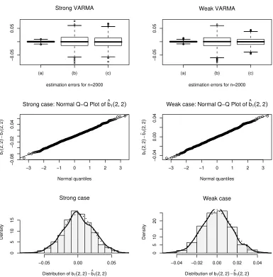
in the weak case. Model (9) is a VARMA(1,1) model in echelon form. The noise defined by (11) is a direct extension of a weak noise defined by Romano and Thombs (1996) in the univariate case. The numerical illustrations of this section are made with the free statistical software R (see http://cran.r-project.org/). We simulated N = 1,000 independent trajectories of size
n = 2,000 of Model (9), first with the strong Gaussian noise (10), second with the weak noise (11). Figure 1 compares the distribution of the QMLE in the strong and weak noise cases. The distributions ofaˆ1(2,2)and ˆb1(2,1)
are similar in the two cases, whereas the QMLE ofˆb1(2,2) is more accurate
in the weak case than in the strong one. Similar simulation experiments, not reported here, reveal that the situation is opposite, that is the QMLE is more accurate in the strong case than in the weak case, when the weak noise is defined by ǫi,t=ηi,tηi,t−1 for i= 1,2. This is in accordance with the
[image:15.612.116.496.87.176.2]results of Romano and Thombs (1996) who showed that, with similar noises, the asymptotic variance of the sample autocorrelations can be greater or less than 1 as well (1 is the asymptotic variance for strong white noises).
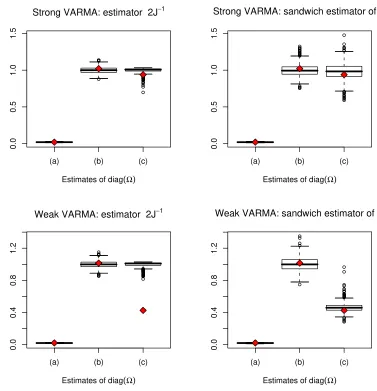
Figure 2 compares the standard estimator Ω = 2 ˆˆ J−1 and the sandwich
estimator Ω = ˆˆ J−1IˆJˆ−1 of the QMLE asymptotic variance Ω. We used the
spectral estimator Iˆ = ˆISP defined in Theorem 4, and the AR order r is
automatically selected by AIC, using the function VARselect() of the vars
R package. In the strong VARMA case we know that the two estimators are consistent. In view of the two top panels of Figure 2, it seems that the sand-wich estimator is less accurate in the strong case. This is not surprising be-cause the sandwich estimator is more robust, in the sense that this estimator continues to be consistent in the weak VARMA case, contrary to the stan-dard estimator. It is clear that in the weak casenVarnˆb1(2,2)−b1(2,2)
o2
is better estimated byΩˆSP(3,3)(see the box-plot (c) of the right-bottom panel
of Figure 2) than by 2 ˆJ−1(3,3)(box-plot (c) of the left-bottom panel). The
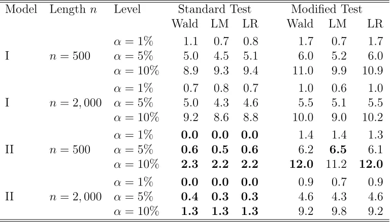
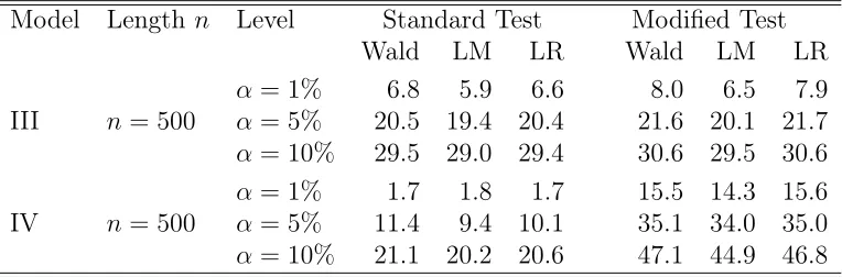
Table 1 displays the empirical sizes of the standard Wald, LM and LR tests, and that of the modified versions proposed in Section 5. For the nomi-nal level α= 5%, the empirical size over theN = 1,000independent replica-tions should vary between the significant limits 3.6% and 6.4% with proba-bility 95%. For the nominal level α= 1%, the significant limits are 0.3% and 1.7%, and for the nominal level α = 10%, they are 8.1% and 11.9%. When the relative rejection frequencies are outside the significant limits, they are displayed in bold type in Table 1. For the strong VARMA model I, all the relative rejection frequencies are inside the significant limits. For the weak VARMA model II, the relative rejection frequencies of the standard tests are definitely outside the significant limits. Thus the error of first kind is well controlled by all the tests in the strong case, but only by modified versions of the tests in the weak case. Table 2 shows that the powers of all the tests are very similar in the Model III case. The same is also true for the two modified tests in the Model IV case. The empirical powers of the standard tests are hardly interpretable for Model IV, because we have already seen in Table 1 that the standard versions of the tests do not well control the error of first kind in the weak VARMA framework.
From these simulation experiments and from the asymptotic theory, we draw the conclusion that the standard methodology, based on the QMLE, allows to fit VARMA representations of a wide class of nonlinear multivariate time series. This standard methodology, including in particular the signif-icance tests on the parameters, needs however to be adapted to take into account the possible lack of independence of the errors terms. In future works, we intent to study how the existing identification (see e.g. Nsiri and Roy, 1996) and diagnostic checking (see e.g. Duchesne and Roy, 2004) pro-cedures should be adapted in the weak VARMA framework considered in the present paper.
A. Technical proofs
We begin with a lemma useful to show the identifiability of ϑ0.
Lemma 1. Assume that Σ0 is non singular and that A5 holds
true. If A−01B0Bϑ−1(L)Aϑ(L)Xt = A−001B00ǫt with probability one and
A−01B0ΣB0′A−1
′
0 =A−001B00Σ0B00′ A−1
′
00 , then ϑ=ϑ0.
Proof: Let ϑ 6= ϑ0. Assumption A5 implies that either A0−1B0ΣB0′A−1
′
0 6=
A−001B00Σ0B00′ A−1
′
Table 1: Empirical size of standard and modified tests: relative frequencies (in %) of rejection of H0 :b1(2,2) = 0. The number of replications is N = 1000.
Model Length n Level Standard Test Modified Test Wald LM LR Wald LM LR
α= 1% 1.1 0.7 0.8 1.7 0.7 1.7
I n = 500 α= 5% 5.0 4.5 5.1 6.0 5.2 6.0
α= 10% 8.9 9.3 9.4 11.0 9.9 10.9
α= 1% 0.7 0.8 0.7 1.0 0.6 1.0 I n = 2,000 α= 5% 5.0 4.3 4.6 5.5 5.1 5.5
α= 10% 9.2 8.6 8.8 10.0 9.0 10.2
α= 1% 0.0 0.0 0.0 1.4 1.4 1.3
II n = 500 α= 5% 0.6 0.5 0.6 6.2 6.5 6.1
α= 10% 2.3 2.2 2.2 12.0 11.2 12.0
α= 1% 0.0 0.0 0.0 0.9 0.7 0.9 II n = 2,000 α= 5% 0.4 0.3 0.3 4.6 4.3 4.6
α= 10% 1.3 1.3 1.3 9.2 9.8 9.2
I: Strong VARMA(1,1) model (9)-(10) with ϑ0 = (0.95,2,0)
II: Weak VARMA(1,1) model (9)-(11) with ϑ0 = (0.95,2,0)
i0 >0 and
A−01B0Bϑ−1(z)Aϑ(z)−A−001B00Bϑ−01(z)Aϑ0(z) =
∞
X
i=i0
Cizi.
By contradiction, assume that A−01B0Bϑ−1(L)Aϑ(L)Xt = A−001B00ǫt =
A−001B00B−ϑ01(L)Aϑ0(L)Xt with probability one. This implies that there exists
λ 6= 0such that λ′X
t−i0 is almost surely a linear combination of the
compo-nents of Xt−i, i > i0. By stationarity, it follows that λ′Xt is almost surely a
linear combination of the components of Xt−i, i > 0. Thus λ′ǫt = 0 almost
surely, which is impossible when the varianceΣ0 ofǫtis positive definite. ✷
Proof of Theorem 1: Note that, due to the initial conditions, {˜et(ϑ)}
is not stationary, but can be approximated by the stationary ergodic process
Table 2: Empirical power of standard and modified tests: relative frequencies (in %) of rejection of H0:b1(2,2) = 0. The number of replications isN = 1000.
Model Length n Level Standard Test Modified Test Wald LM LR Wald LM LR
α= 1% 6.8 5.9 6.6 8.0 6.5 7.9
III n= 500 α= 5% 20.5 19.4 20.4 21.6 20.1 21.7
α= 10% 29.5 29.0 29.4 30.6 29.5 30.6
α= 1% 1.7 1.8 1.7 15.5 14.3 15.6
IV n= 500 α= 5% 11.4 9.4 10.1 35.1 34.0 35.0
α= 10% 21.1 20.2 20.6 47.1 44.9 46.8 III: Strong VARMA(1,1) model (9)-(10) with ϑ0 = (0.95,2,0.05)
IV: Weak VARMA(1,1) model (9)-(11) with ϑ0 = (0.95,2,0.05)
From an extension of Lemma 1 in FZ, it is easy to show that
supϑ∈Θke˜t(ϑ)−et(ϑ)k → 0almost surely at an exponential rate, as t→ ∞.
We thus have
˜
ℓn(ϑ) oP=(1) ℓn(ϑ) := 1
n
n
X
t=1
lt(ϑ) as n→ ∞,
where
lt(ϑ) =dlog(2π) + log det Σe+et′(ϑ)Σ−e1et(ϑ).
Now the ergodic theorem shows that almost surely
ℓn(ϑ) → dlog(2π) +Q(ϑ),
where Q(ϑ) = log det Σe+Ee′1(ϑ)Σ−e1e1(ϑ). We have
Q(ϑ) = E{e1(ϑ0)}′Σ−e1{e1(ϑ0)}+ log det Σe
+E{e1(ϑ)−e1(ϑ0)}′Σ−e1{e1(ϑ)−e1(ϑ0)}
+2E{e1(ϑ)−e1(ϑ0)}′Σ−e1e1(ϑ0).
The last expectation is null because the linear innovation et = et(ϑ0) is
combinations of the Xu for u < t), and because {et(ϑ)−et(ϑ0)} belongs to
this linear past Ht−1. Moreover
Q(ϑ0) = log det Σe0+Ee′1(ϑ0)Σ−e01e1(ϑ0)
= log det Σe0+ Tr Σ−e01Ee1(ϑ0)e′1(ϑ0) = log det Σe0+d.
Thus
Q(ϑ)−Q(ϑ0)≥Tr Σe−1Σe0−log det Σ−e1Σe0 −d ≥0 (13)
using the elementary inequality Tr(A−1B) − log det(A−1B) ≥
Tr(A−1A) − log det(A−1A) = d for all symmetric positive semi-definite
matrices of order d×d. At least one of the two inequalities in (13) is strict, unless if e1(ϑ) =e1(ϑ0)with probability 1 andΣe = Σe0, which is equivalent
toϑ=ϑ0 by Lemma 1. The rest of the proof relies on standard compactness
arguments, as in Theorem 1 of FZ. ✷
Proof of Theorem 2: In view of Theorem 1 andA6, we have almost surely
ˆ
ϑn → ϑ0 ∈
◦
Θ. Thus ∂ℓ˜n( ˆϑn)/∂ϑ = 0 for sufficiently large n, and a Taylor
expansion gives
0oP=(1)√n∂ℓn(ϑ0) ∂ϑ +
∂2ℓn(ϑ 0)
∂ϑ∂ϑ′
√
nϑˆn−ϑ0
, (14)
using arguments given in FZ (proof of Theorem 2). The proof then directly follows from Lemma 3 and Lemma 5 below. ✷
We first state elementary derivative rules, which can be found in Appendix A.13 of Lütkepohl (1993).
Lemma 2. If f(A) is a scalar function of a matrix A whose elements aij are function of a variable x, then
∂f(A)
∂x =
X
i,j
∂f(A)
∂aij
∂aij
∂x =Tr
∂f(A)
∂A′
∂A ∂x
. (15)
When A is invertible, we also have
∂log|det(A)|
∂A′ = A
−1 (16)
∂Tr(CA−1B)
∂A′ = −A
−1BCA−1 (17)
∂Tr(CAB)
Lemma 3. Under the assumptions of Theorem 2, almost surely
∂2ℓn(ϑ 0)
∂ϑ∂ϑ′ →J, where J is invertible.
Proof of Lemma 3: Let ϑ= (ϑ1, . . . , ϑk0)
′. In view of (15), (16) and (17),
for all i∈ {1, . . . , k0}, we have
∂lt(ϑ)
∂ϑi
=Tr
Σ−e1
∂Σe
∂ϑi −
Σ−e1et(ϑ)e′t(ϑ)Σ−e1
∂Σe
∂ϑi
+ 2∂e ′ t(ϑ)
∂ϑi
Σ−e1et(ϑ). (19)
Using the previous relations and (18), for all i, j ∈ {1, . . . , k0}, we have
∂2l
t(ϑ)
∂ϑi∂ϑj
= Tr
Σ−e1
∂2Σ
e
∂ϑi∂ϑj − Σ−e1
∂Σe
∂ϑi Σ−e1
∂Σe
∂ϑj −
Σ−e1et(ϑ)e′t(ϑ)Σ−e1
∂2Σ
e
∂ϑi∂ϑj
+Σ−e1∂Σe
∂ϑi
Σ−e1et(ϑ)e′t(ϑ)Σ−e1
∂Σe
∂ϑj
+ Σ−e1et(ϑ)e′t(ϑ)Σ−e1
∂Σe
∂ϑi
Σ−e1∂Σe
∂ϑj
−Σ−e1∂Σe
∂ϑi
Σ−e1∂et(ϑ)e ′ t(ϑ)
∂ϑj
+ 2∂
2e′ t(ϑ)
∂ϑi∂ϑj
Σ−e1et(ϑ)
+2∂e ′ t(ϑ)
∂ϑi
Σ−e1∂et(ϑ)
∂ϑj − 2Tr
Σ−e1et(ϑ)∂e ′ t(ϑ)
∂ϑi
Σ−e1∂Σe
∂ϑj
. (20)
Using Eete′t = Σe, Eet = 0, the uncorrelatedness between et and the linear
past Ht−1, ∂et(ϑ0)/∂ϑi ∈ Ht−1, and∂2et(ϑ0)/∂ϑi∂ϑj ∈Ht−1, we have
E∂
2lt(ϑ 0)
∂ϑi∂ϑj
= Tr
Σ−e01∂Σe(ϑ0)
∂ϑi
Σ−e01∂Σe(ϑ0)
∂ϑj
+ 2E∂e
′ t(ϑ0)
∂ϑi
Σ−e01∂et(ϑ0)
∂ϑj
= J(i, j). (21)
The ergodic theorem and the next lemma conclude. ✷
Lemma 4. Under the assumptions of Theorem 2, the matrix
J =E∂
2lt(ϑ 0)
Proof of Lemma 4: In view of (21), we haveJ =J1+J2, where
J2 = 2E
∂e′ t(ϑ0)
∂ϑ Σ
−1
e0
∂et(ϑ0)
∂ϑ′
and
J1(i, j) = Tr
Σ−e01/2∂Σe(ϑ0)
∂ϑi
Σe−01/2Σe−01/2∂Σe(ϑ0)
∂ϑj
Σ−e01/2
=h′ ihj,
with
hi = (Σ−1/2
e0 ⊗Σ
−1/2
e0 )di, di =vec
∂Σe(ϑ0)
∂ϑi
.
In the previous derivations, we used the well-known relations Tr(A′B) = (vecA)′vecB and vec(ABC) = (C′⊗A)vecB. Note that the matrices J, J
1
and J2 are semi-definite positive. IfJ is singular, then there exists a vector
c = (c1, . . . , ck
0)
′ 6= 0 such that c′J
1c =c′J2c = 0. Since Σ−e01/2⊗Σ
−1/2
e0 and
Σ−e01 are definite positive, we have c′J
1c= 0if and only if
k0
X
k=1
ckdk = k0
X
k=1
ckvec
∂Σe(ϑ0)
∂ϑk
= 0 (22)
and c′J2c = 0 if and only if Pk0
k=1ck
∂et(ϑ0)
∂ϑk = 0 a.s. Differentiating the two
sides of the reduced form representation (3), the latter equation yields the VARMA(p−1, q−1) equation Pp
i=1A∗iXt−i =Ppj=1Bj∗et−j. The
identifia-bility assumption A5 excludes the existence of such a representation. Thus
A∗i = k0
X
k=1
ck
∂A−01Ai
∂ϑk
(ϑ0) = 0, Bj∗ = k0
X
k=1
ck
∂A−01BjB0−1A0
∂ϑk
(ϑ0) = 0. (23)
It can be seen that (22) and (23), for i = 1, . . . , p and j = 1, . . . , q, are equivalent to M ϑ0 c = 0. We conclude from A8. ✷
Lemma 5. Under the assumptions of Theorem 2,
√
n∂ℓn(ϑ0) ∂ϑ
L
Proof of Lemma 5: In view of (12), we have
∂et(ϑ0)
∂ϑi =
∞
X
ℓ=1
d′ℓet−ℓ, (24)
where the sequence of matricesdℓ=dℓ(i)is such thatkdℓk →0at a geometric
rate as ℓ→ ∞. By (19), we have for all m ∂lt(ϑ0)
∂ϑi
= Tr
Σ−e01
Id−ete′tΣ−e01
∂Σe(ϑ0)
∂ϑi
+ 2∂e ′ t(ϑ0)
∂ϑi
Σ−e01et = Yt,m,i+Zt,m,i
where
Yt,m,i = Tr
Σ−1
e0
Id−ete′tΣ−e01
∂Σe(ϑ0)
∂ϑi + 2 m X ℓ=1 e′
t−ℓd′ℓΣ−e01et
Zt,m,i = 2 ∞
X
ℓ=m+1
e′t−ℓd′ℓΣ−e01et.
LetYt,m = (Yt,m,1, . . . , Yt,m,k0)
′
andZt,m = (Zt,m,1, . . . , Yt,m,k0)
′
. The processes
(Yt,m)tand(Zt,m)tare stationary and centered. Moreover, under Assumption A7 and m fixed, the process Y = (Yt,m)t is strongly mixing, with mixing coefficientsαY(h)≤αǫ(max{0, h−m}). Applying the central limit theorem
(CLT) for mixing processes (see Herrndorf, 1984) we directly obtain
1 √ n n X t=1
Yt,m → NL (0, Im), Im = ∞
X
h=−∞
Cov (Yt,m, Yt−h,m).
As in FZ Lemma 3, one can show that I = limm→∞Im exists. Since
kZt,mk2 → 0 at an exponential rate when m → ∞, using the arguments
given in FZ Lemma 4, one can show that
lim
m→∞lim supn→∞ P
(
n−1/2
n X t=1 Zt,m > ε )
= 0 (25)
for everyε >0. From a standard result (seee.g. Brockwell and Davis, 1991, Proposition 6.3.9), we deduce that
1 √ n n X t=1
∂lt(ϑ0)
∂ϑ = 1 √ n n X t=1
Yt,m+ 1 √ n n X t=1 Zt,m L
which completes the proof. ✷
Proof of Theorem 3: Note that
˜
ℓn(ϑ) = 1
n
n
X
t=1
˜
lt(ϑ), ˜lt(ϑ) =dlog(2π) + log det Σe+ ˜e′t(ϑ)Σ−e1˜et(ϑ).
Under the assumption of the theorem, ∂e˜′
t(ϑ)/∂ϑ(2) = 0, and (19) yields
∂˜lt( ˆϑn)
∂ϑi
=Tr
"
ˆ Σ−1
e
n
Id−˜et( ˆϑ(1)n )˜e′t( ˆϑ(1)n ) ˆΣ−e1
o∂Σ
e( ˆϑn)
∂ϑi
#
for i = k1 + 1, . . . k0, with Σeˆ such that ϑˆ(2)n = Dvec ˆΣe. Assumption A6
entails that the first order condition∂ℓ˜n( ˆϑn)/∂ϑ(2) = 0 is satisfied forn large
enough. We then have
ˆ
Σe=n−1
n
X
t=1
˜
et( ˆϑ(1)n )˜e′t( ˆϑ(1)n )
and
˜
ℓn( ˆϑn) = dlog(2π) + log det ˆΣe+d,
because
1
n
n
X
t=1
˜
et′( ˆϑ(1)n ) ˆΣe−1˜et( ˆϑ(1)n ) =Tr
"
1
n
n
X
t=1
˜
et( ˆϑ(1)n )˜e′t( ˆϑ(1)n ) ˆΣ−e1
#
=d.
The conclusion follows. ✷
References
[1] Andrews, D.W.K. (1991) Heteroskedasticity and autocorrelation consis-tent covariance matrix estimation. Econometrica 59, 817–858.
[2] Berk, K.N. (1974) Consistent Autoregressive Spectral Estimates.Annals of Statistics, 2, 489–502.
[3] Brockwell, P.J. and Davis, R.A. (1991)Time series: theory and methods.
[4] den Hann, W.J. and Levin, A. (1997) A Practitioner’s Guide to Robust Covariance Matrix Estimation. In Handbook of Statistics15, Rao, C.R. and G.S. Maddala (eds), 291–341.
[5] Duchesne, P. and Roy, R. (2004) On consistent testing for serial corre-lation of unknown form in vector time series models. Journal of Multi-variate Analysis 89, 148–180.
[6] Dufour, J-M., and Pelletier, D. (2005) Practical methods for modelling weak VARMA processes: identification, estimation and specification with a macroeconomic application. Technical report, Département de sciences économiques and CIREQ, Université de Montréal, Montréal, Canada.
[7] Dunsmuir, W.T.M. and Hannan, E.J. (1976) Vector linear time series models, Advances in Applied Probability 8, 339–364.
[8] Fan, J. and Yao, Q. (2003) Nonlinear time series: Nonparametric and parametric methods. Springer Verlag, New York.
[9] Francq, C. and Raïssi, H. (2007) Multivariate Portmanteau Test for Autoregressive Models with Uncorrelated but Nonindependent Errors,
Journal of Time Series Analysis 28, 454–470.
[10] Francq, C., Roy, R. and Zakoïan, J-M. (2005) Diagnostic checking in ARMA Models with Uncorrelated Errors, Journal of the American Sta-tistical Association 100, 532–544.
[11] Francq, C. and Zakoïan, J-M. (1998) Estimating linear representations of nonlinear processes, Journal of Statistical Planning and Inference68, 145–165.
[12] Francq, and Zakoïan, J-M. (2005) Recent results for linear time series models with non independent innovations. In Statistical Modeling and Analysis for Complex Data Problems, Chap. 12 (eds P.Duchesne and
B. Rémillard). New York: Springer Verlag, 137–161.
[14] Hannan, E.J. (1976) The identification and parametrization of ARMAX and state space forms, Econometrica 44, 713–723.
[15] Hannan, E.J. and Deistler, M. (1988) The Statistical Theory of Linear Systems John Wiley, New York.
[16] Hannan, E.J., Dunsmuir, W.T.M. and Deistler, M. (1980) Estimation of vector ARMAX models, Journal of Multivariate Analysis 10, 275–295.
[17] Hannan, E.J. and Rissanen (1982) Recursive estimation of mixed of Autoregressive Moving Average order, Biometrika 69, 81–94.
[18] Herrndorf, N. (1984) A Functional Central Limit Theorem for Weakly Dependent Sequences of Random Variables. The Annals of Probability
12, 141–153.
[19] Imhof, J.P. (1961) Computing the distribution of quadratic forms in normal variables. Biometrika 48, 419–426.
[20] Kascha, C. (2007) A Comparison of Estimation Methods for Vector Au-toregressive Moving-Average Models. ECO Working Papers, EUI ECO 2007/12, http://hdl.handle.net/1814/6921.
[21] Lütkepohl, H. (1993) Introduction to multiple time series analysis.
Springer Verlag, Berlin.
[22] Lütkepohl, H. (2005) New introduction to multiple time series analysis.
Springer Verlag, Berlin.
[23] Newey, W.K., and West, K.D. (1987) A simple, positive semi-definite, heteroskedasticity and autocorrelation consistent covariance matrix.
Econometrica 55, 703–708.
[24] Nsiri, S., and Roy, R.] (1996) Identification of refined ARMA echelon form models for multivariate time series. Journal of Multivariate Anal-ysis 56, 207–231.
[26] Rissanen, J. and Caines, P.E. (1979) The strong consistency of maximum likelihood estimators for ARMA processes. Annals of Statistics 7, 297– 315.
[27] Romano, J.L. and Thombs, L.A. (1996) Inference for autocorrelations under weak assumptions, Journal of the American Statistical Associa-tion 91, 590–600.
[28] Tong, H. (1990) Non-linear time series: A Dynamical System Approach,
Clarendon Press Oxford.
[30] van der Vaart, A.W. (1998) Asymptotic statistics, Cambridge University Press, Cambridge.
[30] van der Vaart, A.W. (1998) Asymptotic statistics, Cambridge University Press, Cambridge.
(a) (b) (c)
−0.05
0.05
estimation errors for n=2000
Strong VARMA
(a) (b) (c)
−0.05
0.05
estimation errors for n=2000
Weak VARMA
−3 −2 −1 0 1 2 3
−0.08
−0.02
0.04
Normal quantiles b1
(
2
,
2
)
−
b
^(1
2
,
2
)
Strong case: Normal Q−Q Plot of b^1(2, 2)
−3 −2 −1 0 1 2 3
−0.04
0.00
0.04
Normal quantiles b1
(
2
,
2
)
−
b
^(1
2
,
2
)
Weak case: Normal Q−Q Plot of b^1(2, 2)
Strong case
Distribution of b1(2, 2)−b^1(2, 2)
Density
−0.05 0.00 0.05
0
5
10
15
Weak case
Distribution of b1(2, 2)−b^1(2, 2)
Density
−0.04 −0.02 0.00 0.02 0.04
0
5
10
[image:27.612.106.491.97.488.2]20
Figure 1: QMLE of N = 1,000 independent simulations of the VARMA(1,1) model (9) with size n = 2,000 and unknown parameter ϑ0 = ((a1(2,2), b1(2,1), b1(2,2)) = (0.95,2,0), when the noise is strong (left panels) and when the noise is the weak noise (11) (right panels). Points (a)-(c), in the box-plots of the top panels, display the distribution of the estimation errorsϑˆ(i)−ϑ0(i)fori= 1,2,3. The panels of the middle present the Q-Q plot of the estimatesϑˆ(3) = ˆb1(2,2)of the last parameter. The bottom panels display the
(a) (b) (c)
0.0
0.5
1.0
1.5
Estimates of diag(Ω)
Strong VARMA: estimator 2J−1
(a) (b) (c)
0.0
0.5
1.0
1.5
Estimates of diag(Ω)
Strong VARMA: sandwich estimator of Ω
(a) (b) (c)
0.0
0.4
0.8
1.2
Estimates of diag(Ω)
Weak VARMA: estimator 2J−1
(a) (b) (c)
0.0
0.4
0.8
1.2
Estimates of diag(Ω)
[image:28.612.114.491.105.496.2]Weak VARMA: sandwich estimator of Ω
Figure 2: Comparison of standard and modified estimates of the asymptotic variance Ω
of the QMLE, on the simulated models presented in Figure 1. The diamond symbols represent the mean, over the N = 1,000replications, of the standardized squared errors
n{ˆa1(2,2)−0.95} 2
for (a) (0.02 in the strong and weak cases),nnˆb1(2,1)−2
o2
for (b) (1.02 in the strong case and 1.01 in the strong case) andnnˆb1(2,2)o
2
Estimating structural VARMA models with
uncorrelated but non-independent error terms:
Complementary results that are not submitted
for publication
A. Additional example
Example 2. Denoting by a0i(k, ℓ) and b0i(k, ℓ) the generic elements of the
matrices A0i and B0i, the Kronecker indices are defined by pk = max{i :
a0i(k, ℓ) 6= 0 orb0i(k, ℓ) 6= 0 for some ℓ = 1, . . . , d}. To ensure relatively
parsimonious parameterizations, one can specify an echelon form depending on the Kronecker indices (p1, . . . , pd). The reader is refereed to Lütkepohl
(1993) for details about the echelon form. For instance, a 3-variate ARMA process with Kronecker indices (1,2,0)admits the echelon form
1 0 0
0 1 0
× × 1
Xt−
× × 0
0 × 0
0 0 0
Xt−1−
0 0 0
× × 0
0 0 0
Xt−2
=
1 0 0
0 1 0
× × 1
ǫt−
× × × × × ×
0 0 0
ǫt−1 −
0 0 0
× × ×
0 0 0
ǫt−2
where×denotes an unconstrained element. The variance ofǫt is defined by 6
additional parameters. This echelon form thus corresponds to a parametriza-tion by a vector ϑ of size k0 = 24.
B. Verification of Assumption A8 on Example 1
In this example, we have
Mϑ0 =
α01 α02 σ012 σ012 α03
α01α03+α04 α02α03+α05 σ012 α03 σ012 α203+σ202
.
Thus
Mϑ0=
1 α03 0 0 0 0 0 0
0 0 1 α03 0 0 0 0
0 α01 0 α02 0 σ012 σ012 2α03σ012
0 1 0 0 0 0 0 0
0 0 0 1 0 0 0 0
0 0 0 0 1 α03 α03 α203
0 0 0 0 0 0 0 1
is of full rank k0 = 7.
C. Details on the proof of Theorem 1
Lemma 6. Under the assumptions of Theorem 1, we have
sup ϑ∈Θk
˜
et(ϑ)−et(ϑ)k ≤Kρt,
whereρis a constant belonging to[0,1), andK >0is measurable with respect to the σ-field generated by {Xu, u≤0}.
Proof of Lemma 6: We have
et(ϑ) =Xt− p
X
i=1
A−01AiXt−i+ q
X
i=1
A−01BiB0−1A0et−i(ϑ) ∀t∈Z, (26)
and
˜
et(ϑ) =Xt− p
X
i=1
A−01AiXt−i+ q
X
i=1
A−01BiB0−1A0˜et−i(ϑ) t = 1, . . . , n (27)
with the initial values e˜0(ϑ) =· · ·= ˜e1−q(ϑ) =X0 =· · ·=X1−p = 0. Let
et(ϑ) =
et(ϑ)
et−1(ϑ)
...
et−q+1(ϑ)
, ˜et(ϑ) =
˜
et(ϑ) ˜
et−1(ϑ)
...
˜
et−q+1(ϑ)
.
From (26) and (27), we have
et(ϑ) =bt+Cet−1(ϑ) ∀t∈Z,
and
˜
et(ϑ) = ˜bt+Ce˜
t−1(ϑ) t= 1, . . . , n,
where
C =
A−01B1B0−1A0 · · · A−01BqB0−1A0
I(q−1)d 0(q−1)d
, bt=
Xt−Ppi=1A
−1
˜
bt=bt for t > p,˜bt = 0qd for t≤0, and
˜b t =
Xt−Pt−i=11A−01AiXt−i 0d
...
0d
for t= 1, . . . , p.
Writing dt(ϑ) =et(ϑ)−e˜t(ϑ), we obtain for t > p,
dt(ϑ) = Cd
t−1(ϑ) =Ct−pdp(ϑ) = Ct−pnb
p−˜bp
+Cb
p−1−˜bp−1
+· · ·+Cp−1b
1−˜b1
o
+Cpb
0.
Note that C is the companion matrix of the polynomial
P(z) =Id− q
X
i=1
A−01BiB0−1A0zi =A−01Bϑ(z)B0−1A0.
By A2, the zeroes of P(z) are of modulus strictly greater than one:
P(z) = 0 ⇒ |z|>1 (28)
By a well-known result on companion matrices, (28) is equivalent to ρ(C)<
1, where ρ(C) denote the spectral radius of C. By the compactness of Θ, we thus have
sup ϑ∈Θ
ρ(C)<1.
We thus have
sup ϑ∈Θk
dt(ϑ)k ≤Kρt,
whereK andρare as in the statement of the lemma. The conclusion follows. ✷
Lemma 7. Under the assumptions of Theorem 1, we have
sup ϑ∈Θ
˜
ℓn(ϑ)−ℓn(ϑ)
=o(1)
Proof of Lemma 7: We have
˜
ℓn(ϑ)−ℓn(ϑ) = 1
n
n
X
t=1
{e˜t(ϑ)−et(ϑ)}′Σ−e1e˜t(ϑ) +e′t(ϑ)Σ−e1{e˜t(ϑ)−et(ϑ)}.
In the proof of this lemma and in the rest on the paper, the letters K and ρ
denote generic constants, whose values can be modified along the text, such that K >0 and 0< ρ <1. By Lemma 6,
sup ϑ∈Θ
ℓ˜n(ϑ)−ℓn(ϑ)
≤
K n
n
X
t=1
ρt
sup ϑ∈Θk
et(ϑ)k+ sup ϑ∈Θk
˜
et(ϑ)k
≤ Kn
n
X
t=1
ρtsup ϑ∈Θk
et(ϑ)k (29)
In view of (26), and using A1 and the compactness of Θ, we have
et(ϑ) =Xt+ ∞
X
i=1
Ci(ϑ)Xt−i, sup ϑ∈Θk
Ci(ϑ)k ≤Kρi. (30)
We thus have Esupϑ∈Θket(ϑ)k<∞, and the Markov inequality entails
∞
X
t=1
P
ρtsup ϑ∈Θk
et(ϑ)k> ε
≤Esup ϑ∈Θk
et(ϑ)k ∞
X
t=1
ρt
ε <∞.
By the Borel-Cantelli theorem, ρtsup
ϑ∈Θket(ϑ)k → 0 almost surely as
t → ∞. The Cesàro theorem implies that the right-hand side of (29) converges to zero almost surely. ✷
Lemma 8. Under the assumptions of Theorem 1, any ϑ 6= ϑ0 has a
neigh-borhood V(ϑ) such that
lim inf
n→∞ ϑ∗∈Vinf(ϑ)
˜
ℓn(ϑ∗)> El1(ϑ0), a.s. (31)
Moreover for any neighborhood V(ϑ0) of ϑ0 we have
lim sup n→∞
inf ϑ∗∈V(ϑ0)
˜
Proof of Lemma 8: For any ϑ ∈ Θ and any positive integer k, let Vk(ϑ)
be the open ball with center ϑ and radius 1/k. Using Lemma 7, we have
lim inf
n→∞ ϑ∗∈Vkinf(ϑ)∩Θ
˜
ℓn(ϑ∗) ≥ lim inf
n→∞ ϑ∗∈Vkinf(ϑ)∩Θℓn(ϑ
∗)
−lim sup n→∞
sup ϑ∈Θ|
ℓn(ϑ)−ℓ˜n(ϑ)|
≥ lim inf n→∞ n
−1
n
X
t=1
inf
ϑ∗∈Vk(ϑ)∩Θlt(ϑ
∗)
= E inf
ϑ∗∈Vk(ϑ)∩Θl1(ϑ
∗)
For the last equality we applied the ergodic theorem to the ergodic stationary process
infϑ∗∈Vk(ϑ)∩Θℓt(ϑ∗)
t. By the Beppo-Levi theorem, whenkincreases
to∞,Einfϑ∗∈Vk(ϑ)∩Θl1(ϑ∗)increases toEl1(ϑ).BecauseEl1(ϑ) =dlog(2π)+ Q(ϑ), the discussion which follows (13) entails El1(ϑ) > El1(ϑ0), and (31)
follows.
To show (32), it suffices to remark that Lemma 7 and the ergodic theorem entail
lim sup n→∞
inf ϑ∗∈V(ϑ)∩Θ
˜
ℓn(ϑ∗) ≤ lim sup n→∞
inf
ϑ∗∈V(ϑ)∩Θℓn(ϑ
∗) + lim sup
n→∞ sup ϑ∈Θ|
ℓn(ϑ)−ℓ˜n(ϑ)|
≤ lim sup n→∞ n
−1
n
X
t=1
lt(ϑ0)
= El1(ϑ0).
✷
The proof of Theorem 1 is completed by the arguments of Wald (1949). More precisely, the compact set Θ is covered by a neighborhoodV(ϑ0) of ϑ0
and a finite number of neighborhoods V(ϑ1), . . . , V(ϑk) satisfying (31) with
ϑ replaced by ϑi, i = 1, . . . , k. In view of (31) and (32), we have almost
surely
inf ϑ∈Θ
˜
ℓn(ϑ) = min
i=0,1,...,kϑ∈Vinf(ϑi)∩Θ
˜
ℓn(ϑ) = inf ϑ∈V(ϑ0)∩Θ
˜
ℓn(ϑ)
for n large enough. Since the neighborhood V(ϑ0) can be chosen arbitrarily
D. Details on the proof of Theorem 2
Lemma 9. Under the assumptions of Theorem 2, we have
√ nsup ϑ∈Θ
∂ℓ˜n(ϑ)
∂ϑ −
∂ℓn(ϑ)
∂ϑ
=oP(1).
Proof of Lemma 9: Similar to (30), Assumption A1 entails that, for
k = 1, . . . , k0,
∂et(ϑ)
∂ϑk =
∞
X
i=1
Ci(k)(ϑ)Xt−i,
∂e˜t(ϑ)
∂ϑk =
t−1
X
i=1
Ci(k)(ϑ)Xt−i, (33)
Ci(k)(ϑ) = ∂Ci(ϑ)
∂ϑk , sup ϑ∈Θ C
(k)
i (ϑ)
≤Kρ
i. (34)
Similar to Lemma 6, we then have
sup ϑ∈Θ
∂e˜t(ϑ)
∂ϑ′ −
∂et(ϑ)
∂ϑ′
≤
Kρt. (35)
Using (19), we have
√
n
(
∂ℓ˜n(ϑ)
∂ϑk −
∂ℓn(ϑ)
∂ϑk
)
=a1 +a2,
with
a1 =
2 √ n n X t=1 ∂e′ t(ϑ)
∂ϑk −
∂˜e′ t(ϑ)
∂ϑk
Σ−e1et(ϑ) +∂e˜ ′ t(ϑ)
∂ϑk
Σ−e1(et(ϑ)−e˜t(ϑ))
a2 = Tr
Σ−e1
{e˜t(ϑ)−et(ϑ)}e˜′t(ϑ) +et(ϑ){˜et(ϑ)−et(ϑ)}′
Σ−e1∂Σe
∂ϑk
.
From Lemma 6 and (35), it follows that
|a1|+|a2| ≤
K √ n n X t=1
bt, bt=ρt
sup ϑ∈Θ
∂et(ϑ)
∂ϑk + sup ϑ∈Θk
et(ϑ)k+Kρt
.
In view of (30) and (33)-(34), we have
Esup ϑ∈Θ
∂et(ϑ)
∂ϑk
By the Markov inequality, for all ε >0 we thus have
P √K n
n
X
t=1
bt> ε
!
≤ K
ε√n
n
X
t=1
ρt→0,
and the conclusion follows. ✷
Lemma 10. Under the assumptions of Theorem 2, (14) holds, that is
0oP=(1)√n∂ℓn(ϑ0) ∂ϑ +
∂2ℓ
n(ϑ0)
∂ϑ∂ϑ′
√
nϑˆn−ϑ0
.
Proof of Lemma 10: By Lemma 9 and already given arguments, we have
0 =√nℓ˜n( ˆϑn) ∂ϑ =
√
nℓn( ˆϑn) ∂ϑ +
√
nℓ˜n( ˆϑn) ∂ϑ −
√
nℓn( ˆϑn) ∂ϑ
oP(1)
= √nℓn( ˆϑn) ∂ϑ .
Taylor expansions of the functions ∂ℓn(·)/∂ϑi aroundϑ0 give
√
nℓn( ˆϑn) ∂ϑ =
√
n∂ℓn(ϑ0) ∂ϑ +
∂2ℓn(ϑ∗ i)
∂ϑi∂ϑj
√
nϑˆn−ϑ0
,
for some ϑ∗
i between ϑˆn and ϑ0.
From (20) and Lemma 2, one can see that the random terms involved in
∂3l
t(ϑ)
∂ϑk1∂ϑk2∂ϑk3
are linear combinations of the elements of the following matrices
et(ϑ)e′t(ϑ), et(ϑ)
∂e′ t(ϑ)
∂ϑki
, et(ϑ)
∂2e′ t(ϑ)
∂ϑki∂ϑkj
,
∂et(ϑ)
∂ϑki
∂e′ t(ϑ)
∂ϑkj
, ∂et(ϑ) ∂ϑki
∂2e′ t(ϑ)
∂ϑkj∂ϑkℓ
, et(ϑ) ∂
3e′ t(ϑ)
∂ϑki∂ϑkj∂ϑkℓ
.
Since all these matrices have finite expectations uniformly inϑ ∈Θ, we have
Esup ϑ∈Θ
∂3lt(ϑ)
∂ϑk1∂ϑk2∂ϑk3
for all k1, k2, k3 ∈ {1, . . . , k0}. Now a second Taylor expansion yields
∂2ℓn(ϑ∗ i)
∂ϑi∂ϑj
= ∂
2ℓn(ϑ 0)
∂ϑi∂ϑj
+ ∂
∂ϑ′
∂2ℓn(ϑ∗)
∂ϑi∂ϑj
(ϑ∗i −ϑ0)
= ∂
2ℓn(ϑ 0)
∂ϑi∂ϑj
+o(1) a.s.
using the ergodic theorem, (36) and the almost sure convergence ofϑ∗ i toϑ0.
The proof is complete. ✷
Now we need the following covariance inequality obtained by Davydov (1968).2
Lemma 11 (Davydov (1968)). Letp,q andrthree positive numbers such that p−1+q−1+r−1 = 1. Davydov (1968) showed that
|Cov(X, Y)| ≤K0kXkpkYkq[α{σ(X), σ(Y)}]1/r, (37)
where kXkp
p = EXp, K0 is an universal constant, and α{σ(X), σ(Y)}
de-notes the strong mixing coefficient between the σ-fields σ(X) and σ(Y) gen-erated by the random variables X and Y, respectively.
Lemma 12. Under the assumptions of Theorem 2, (25) holds, that is
lim
m→∞lim supn→∞ P
(
n−1/2
n
X
t=1
Zt,m
> ε
)
= 0.
Proof of Lemma 12: Fori= 1, . . . , k0, by stationarity we have
var √1
n
n
X
t=1
Zt,m,i
!
= 1
n
n
X
t,s=1
Cov(Zt,m,i, Zs,m,i)
= 1
n
X
|h|<n
(n− |h|)Cov(Zt,m,i, Zt−h,m,i)
≤
∞
X
h=−∞
|Cov(Zt,m,i, Zt−h,m,i)|.
2Davydov, Y. A. (1968) Convergence of Distributions Generated by Stationary
Because kdℓk ≤Kρℓ, we have
|Zt,m,i| ≤K ∞
X
ℓ=m+1
ρℓke
tkket−ℓk.
Using also Eketk4 <∞, it follows from the Hölder inequality that
sup h |
Cov(Zt,m,i, Zt−h,m,i)|= sup h |
EZt,m,iZt−h,m,i| ≤Kρm. (38)
Let h >0 such that [h/2]> m. Write
Zt,m,i =Zh
−
t,m,i+Zh
+
t,m,i,
where
Zt,m,ih− = 2
[h/2]
X
ℓ=m+1
e′t−ℓd′ℓΣ−e01et, Zh
+
t,m,i = 2 ∞
X
ℓ=[h/2]+1
e′t−ℓd′ℓΣ−e01et.
Note thatZh−
t,m,i belongs to theσ-field generated by{et, et−1, . . . , et−[h/2]}and
thatZt−h,m,i belongs to theσ-field generated by{et−h, et−h−1, . . .}. Note also
that αe(·) = αǫ(·) and that, by A7, E|Zh−
t,m,i|2+ν < ∞ and E|Zt−h,m,i|2+ν <
∞. Lemma 11 then entails that
Cov(Z
h−
t,m,i, Zt−h,m,i)
≤Kα
ν/(2+ν)
ǫ ([h/2]). (39)
By the argument used to show (38), we also have
Cov(Z
h+
t,m,i, Zt−h,m,i)
≤Kρ
hρm. (40)
In view of (38), (39) and (40),
∞
X
h=0
|Cov(Zt,m,i, Zt−h,m,i)| ≤Kρm+K ∞
X
h=m
αν/ǫ (2+ν)(h)→0