The determinants of macroeconomic
volatility: A Bayesian model averaging
approach
Spiliopoulos, Leonidas
18 November 2010
averaging approach
Leonidas Spiliopoulos
Abstract Bayesian model averaging is applied to robustly ascertain the determinants of various
output volatility measures, including the downside semideviation of growth rates. Financial
sophis-tication variables are found to have qualitatively different effects on volatility. The ratio of
govern-ment expenditure to GDP exhibited a significant positive relationship with volatility and the trade
share of GDP was positively related for a balanced dataset of developed and developing countries
between 1960-89, and negatively related for developing countries between 1974-89. Other significant
determinants were the black market premium, civil liberties, political rights, rule of law, and ratios
of short-term debt and taxation to GDP.
Keywords Macroeconomic volatility, Growth, Government policy, Bayesian model averaging,
Model selection
JEL codes C11, C52, E32, E60, F00, O47
1 Introduction
There are numerous reasons why research into the determinants of output volatility is important,
especially for developing countries which exhibit significantly greater output volatility than
devel-oped countries. Volatility in growth rates creates economic uncertainty impacting future growth
rates negatively as first documented in Ramey and Ramey (1995). Also, assuming that agents in
the economy are risk-averse, volatility in growth rates and therefore income produces adverse real
welfare effects. The effects of volatility on welfare can be significant, even reaching 5-10 percent
of consumption (Athanasoulis and Van Wincoop, 2000). A better understanding of the causes of
volatility can lead to more effective government policy that directly addresses the long term,
un-derlying causes of volatility instead of relying only on fiscal policy which is an ex post attempt to
temporarily reduce short-run volatility. Readers are referred to Loayza et al (2007) for an overview
of macroeconomic volatility, possible causes and welfare effects for developing countries.
The macroeconomic literature is rife with econometric studies on the determinants of the growth
rates of economies (Barro and Sala-i-Martin, 1995; Temple, 2000; Levine and Renelt, 1992; Levine
et al, 2000) to name but a few. The initial phase of research focused on specific types or subsets of
variables and their effects on growth rates, for example variables of financial sophistication. These
studies usually attempt to address the issue of robustness of their results in the face of model
specification uncertainty by conditioning on other variables considered to be significant. Despite
this, the majority of studies used relatively small, non-overlapping subsets of variables in the growth
regressions estimated, so that it was common to find disagreement amongst different studies as to
the effect of certain variables upon growth rates.1
The second phase of this research was driven by the application of various econometric
tech-niques designed to specifically address model specification. The first attempt by Levine and Renelt
(1992) was based on a variant of a frequentist approach, Extreme Bounds Analysis (EBA)
recom-mended by Leamer (1983). This involved estimating models of all possible combinations of variables
and concluding that a variable’s relationship with the growth rate is considered robust if at the
extreme bounds the coefficient remains significant and of the same sign. Sala-i-Martin (1997)
re-laxes the strictness of the EBA approach by examining the whole distribution of the estimated
coefficients instead of only their values at the extreme bounds. Kalaitzidakis et al (2002) follow a
1 Of course the conflicting results were not just due to different conditioning sets but also due to the use of different
different approach focusing on the estimated coefficients of models that are well specified according
to non-nested hypothesis tests. With the increase in computational power and associated decrease in
computational cost, the literature turned to either approximate Bayesian techniques (Sala-i-Martin
et al, 2004) or Bayesian Model Averaging (Fernandez et al, 2001) for a more statistically rigorous
analysis of model specification. Finally, Ley and Steel (2009) and Eicher et al (2007) examine the
robustness of Bayesian Model Averaging techniques with respect to the alternative specifications
over priors.
The current state of the literature on the determinants of volatility parallels the first phase of
the growth literature, as it is comprised of a number of studies using very different and specific
subsets of variables with often diametrically opposite conclusions. The effects of financial variables
on growth volatility are addressed in Easterly et al (2001); Denizer et al (2000); Ferreira da Silva
(2002), of trade/openness variables in Frankel and Rose (1998); Anderson et al (1999); Bejan (2006);
Hakura (2007); Di Giovanni and Levchenko (2009); Cavallo (2007), of fiscal policy and government
size in Van den Noord (2000); Fatas and Mihov (2001); Virén (2005) and of the role of institutions
in Mobarak (2005); Malik and Temple (2009).
It is our contention that the evolution of this literature now calls for studies that specifically
address model specification and uncertainty. Hence, this paper will use the latest Bayesian Model
Averaging techniques in order to ascertain the robustness of a large set of possible determinants of
volatility. This paper will also contend that a more relevant measure of volatility is the downside
semideviation (the standard deviation of growth rates below the mean growth over the time period
in question) as risk is more closely associated with the volatility of undesirable outcomes. Finally, the
datasets employed include variables rarely or never investigated in the literature such as measures
of different types of taxation and short/long term government debt.
The expositional structure of the paper follows. A literature review of both theoretical and
empiri-cal work regarding the determinants of volatility follows directly in Section 2. The BMA methodology
is presented in Section 3.1, followed by a discussion of the dataset and of the various measures of
volatility in Section 3.2. The following sections discuss the results using a dataset of 60 countries from
1960-89. Section 4.1 concerns the determinants of downside semideviation volatility, whilst Section
4.2 compares the results with other measures of volatility. The forecasting performance of the BMA
technique is contrasted to that of other modeling techniques in Section 4.3. The determinants of
Section 4.5 investigates the determinants of downside semideviation volatility for a dataset including
the years 1974-89 for 50 countries but with a broader range of explanatory variables than the
pre-vious dataset. Section 5 concludes, whilst Appendix A discusses the robustness of the results with
respect to different priors and Appendix B contains information about the countries and variables
included in the dataset.
2 Literature review
There exists less theoretical research compared to empirical research regarding the determinants of
volatility. Aghion et al (1999) show that if there exists a high degree of physical separation between
investors and savers, and there exist capital market imperfections in the sense that borrowers are
constrained as to how much they can borrow from savers, then the economy may cycle around
its long run steady state growth rate. Hence, according to this theory proxies of financial market
sophistication should be included as determinants of volatility and the relationship between financial
sophistication and volatility is negative. Acemoglu and Zilibotti (1997) in their model show that
in the early states of development of an economy with capital scarcity and investment project
indivisibility, economic agents will not be able to diversify away risk effectively as they can only
invest in a limited number of imperfectly correlated investment projects. The theoretical predictions
of these two papers are supported empirically by Ferreira da Silva (2002) who discovers that financial
variables proxying for financial development and real GDP per capita are negatively related to
output, investment and consumption volatility.
However, a positive relationship between financial sophistication and volatility can also be
de-fended. For example, more sophisticated and larger financial markets can channel more credit to the
economy leading to greater leverage and volatility. Also, if more credit is available then the resulting
lower interest rates will lead to an increase in the average risk of investments in the economy as the
quality of the marginal investments undertaken will be lower.
Easterly et al (2001) find evidence for a non-linear relationship between financial sophistication
and volatility exhibiting both a negative and positive relationship with volatility. The ratio of private
credit to GDP was initially found to reduce volatility up to a certain degree of financial sophistication
but thereafter was found to exacerbate volatility. Also, they find that countries with greater trade
Investigating the link between financial openness and volatility over time Buch et al (2005)
conclude that the relationship is unstable and that the dependence is influenced by the type of
un-derlying shock to the economy e.g. the effect of interest rate volatility is enhanced in open financial
markets, whilst the effect of volatility of government spending is reduced. Equity market
liberaliza-tion is found to be negatively related to both GDP and consumpliberaliza-tion volatility (Bekaert et al, 2006),
although the magnitude of the effect is reduced for a dataset including the South East Asian crisis.
The literature relating trade openness to volatility has not been able to conclusively agree on the
direction of the effect, with many studies also advocating that the effects of openness on volatility
could depend on the wealth of a country. The most prominent argument put forth for a negative
relationship for developing countries is that based on the stylized fact that trading partners’ business
cycles are more synchronized the higher the level of trade between them (Anderson et al, 1999). Since
developing countries that are more open will tend to trade with developed countries, they will benefit
from synchronizing their economies closely to developed countries which exhibit significantly lower
volatility. A further observation is that export sectors will be correlated less with the domestic
economy thereby further reducing volatility. Cavallo (2007) argues that more open countries are
deemed to be more creditworthy and therefore are less credit-constrained allowing them greater
access to foreign capital with which to smooth fluctuations. This argument is especially relevant to
developing countries which tend to be more constrained in raising capital than developed countries.
Finally, wealthier trading partners may be more willing to provide foreign aid to countries in dire
economic circumstances in order to indirectly protect their country’s own trading sectors.
On the other hand, Bejan (2006) finds that openness is positively related to volatility for
devel-oping countries and contends that this is mainly due to increased exposure to terms of trade risk.
Hakura (2007) argues that a positive relationship occurs because government spending is volatile if a
government faces significant budget restrictions. Also, developing countries may have to specialize in
relatively fewer industries than developed countries leading to non-diversified exports and increased
vulnerability to industry-specific demand shocks. Using industry data in a cross-section of countries
Di Giovanni and Levchenko (2009) conclude that the relationship between volatility and trade
open-ness is positive, with the magnitude of the effect five times higher for a typical developing nation
compared to a developed nation. They find that the negative effect on volatility due to the export
effect of the other two channels, increased volatility due to specialization and exposure to global
shocks.
Using a panel data set of 175 countries from 1950-2002 Kim (2007) distinguishes between openness
and external risk finding an insignificant effect of the former on volatility but a significant effect of
the latter. Cavallo (2007) finds that contrary to the majority of the literature the link between trade
openness is negative after conditioning for the effects of exposure to larger terms of trade risk for
more open economies. The explanation put forth for this finding is that openness leads to a reduction
in volatility propagated through financial channels.
The size of government is often assumed to be a proxy for the degree of automatic stabilisers (such
as transfer payments and progressive taxes systems) in an economy as the two are highly correlated
according to Van den Noord (2000), who conclude that automatic fiscal stabilisers contributed to
a decrease in cyclical volatility in the 1990s. Fatas and Mihov (2001) find a significant negative
relationship between government size and volatility for OECD countries and US states even after
correcting for possible endogeneity. Virén (2005) examines a large sample of 208 countries and finds
a weak or even non-existent effect of government size on volatility. Bejan (2006) finds that for
a pooled sample of developed and developing countries openness increases volatility whereas larger
government leads to a decrease. For developing countries government expenditure and trade openness
both exacerbate volatility. For developed countries greater trade openness and larger government
lead to less volatility. Developing countries may exhibit a positive relationship between government
size and volatility if the former is accompanied by greater volatility in government expenditure.
The link between taxation and volatility is one of the least studied topics. In a sample of OECD
countries Posch (2008) finds statistically and economically significant effects of various types of
taxation on volatility, namely labor and corporate income tax are negatively related to volatility
whilst capital tax is positively related.
Cecchetti et al (2006) concentrate on the stylized fact that volatility in the last twenty years
has been declining, finding that this is primarily due to improved inventory management processes,
financial innovation and increased central bank independence. In a similar paper Kent et al (2005)
discover that less product market regulation and stricter monetary policy have also contributed to
this decline over time.
A non-parametric study of volatility is undertaken in Fiaschi and Lavezzi (2005), concluding that
by the income share of the agricultural sector, and finally is not found to depend on per capita GDP
when other controls are used.
Acemoglu et al (2003) conclude that the fundamental cause of post-war instability arises from
the effects of weak institutions, through channels such as distortionary macroeconomic policies. The
primary results of Mobarak (2005) is that democracy significantly reduces volatility, whilst also
finding that countries with higher income, more outward orientation and lower inflation rates tend
to exhibit less volatility. Malik and Temple (2009) focus on the role of institutions and geography
finding that weaker institutions contribute to volatility and that countries that are more remote
exhibit higher volatility due to a lack of export diversification.
3 Methodology
3.1 BMA methodology
Applications of Bayesian model averaging to the economics field have primarily been made in the
empirical growth regression literature, due to the large number of possible determinants of growth
with little theoretical guidance regarding model/variable selection. Fernandez et al (2001) employ a
Markov chain Monte Carlo Model Composition (MC3) technique to perform BMA for cross-country
growth regressions. In a related paper Ley and Steel (2009) recommend the use of a hierarchical
prior for the prior probability of inclusion of each variable rather than using a fixed probability
which has strong implications for model size, and also argue against the use of the unit information
prior (UIP). Eicher et al (2007) also investigate the effects of twelve different prior distribution
assumptions on the results of BMA methods concluding that although priors affect the selection
of models, the economic impact of the variables as measured by the posterior means of regression
coefficients is very stable across priors. Excellent general discussions of the BMA procedure can be
found in Raftery et al (1997), Hoeting et al (1999) and Montgomery and Nyhan (2010).
Following the notation of Montgomery and Nyhan (2010), let a dependent variable Y be a
vector of sizen×1observations, andX be a matrix of sizen×p, wherepis the number of potential explanatory variables that may influence Y (for simplicity assume that these variables have been
centred at their means so that the constant can be ignored). Define the number of possible model
configurations,q= 2k and let the model spaceM be comprised of[M
1...Mq]. The prior probability
conditioned on a specific model is σ2
| Mk ∼ π(σ2 | Mk). Let Ω = ω1, ..., ωp represent a vector
of zeros and ones for each model Mk denoting which variables are included in said model, then
the conditional distribution βω | σ2, Mk ∼ π(βω | σ2, Mk). If a standard linear regression with
normally distributed errors is assumed then the conditional distribution of the dependent variable is
Y |βω, σ2, Mk ∼N(Xωβω, σ2I). The distribution of the data conditional on the model is given by:
p(Y |Mk) =
� �
p(Y |βω, σ2, Mk)π(βω|σ2, Mk)π(σ2|Mk)dβωdσ2 (1)
Finally, the posterior probability of any model Mk given the dependent data observationsY is:
p(Mk|Y) =
p(Y |Mk)π(Mk)
�q
k=1p(Y |Mk)π(Mk)
(2)
The expected values of the coefficients account for model uncertainty by averaging them across
the entire model space according to:
E(βk |Y) = q
�
k=1
p(Mk|Y)E(βk|Mk, Y) (3)
Computational limitations dictate the use of priors with closed-form solutions for p(Y | Mk)
without the need to sample from the posterior distribution ofMk. Liang et al (2008) suggest imposing
a prior distribution on g thereby also incorporating uncertainty about the g-prior parameter. The results presented in the main sections of this paper assume the hyper-g prior in equation 4, setting the hyper-parameteraequal to 3 as recommended by Liang et al (2008).
π(g) =a−2 2 (1 +g)
a/2
where g >0 (4)
The robustness of the results with respect to the imposition of alternative priors, defined below,
is examined in Appendix A.
1. Zellner’sg-prior (Zellner, 1986) for specific values ofg:
π(βω|Mk, σ2)∼Npω(0, gσ
2 (X�
ωXω)−1) & π(β0, σ 2
2. The Zellner and Siow (1980) prior wheregis distributed according to theΓ(0.5, n/2)distribution. The resulting prior onβω is given by:
π(βω|Mk, σ2)∝
�
N(βω|0, gσ2(Xω�Xω)−1)π(g)dg (6)
3. Finally, an alternative approach is to set the value of g as the maximum marginal likelihood
estimate, constrained to be nonnegative - the local empirical Bayes prior (EB-local) estimates
a different value of g for each model, whereas global empirical Bayes (EB-global) assumes a
common value of gfor all models.
This paper employs the Bayesian Adaptive Sampling methodology advocated in Clyde et al (2009)
which samples without replacement from the model space allowing this algorithm to visit a larger
number of models for a given number of samples. This is shown to be computationally more efficient
than other Markov chain Monte Carlo methods such as theMC3algorithm of Madigan et al (1995);
Raftery et al (1997) and the hybridMC3/Gibbs sampler technique of Clyde et al (1996), whilst also
exhibiting more accurate inclusion probabilities in simulation studies. The software utilized for the
estimation is the freely distributed R-package BAS (Clyde, 2009) implementing the technique in
Clyde et al (2009).
3.2 Datasets and definitions of volatility measures
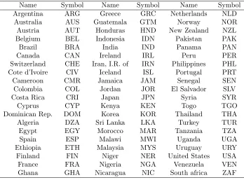
The datasets were compiled from Sala-i-Martin (1997), King and Levine (1993) and the Penn World
Table (Heston et al, 2009) - a list of included countries, explanations and abbreviations of variables
can be found in Appendix B. Independent variables were chosen from the variables used in the
growth literature as there is reason to believe that the same variables may be affecting volatility,
albeit in different ways and for different reasons. A total of 42 possible determinants of volatility
were included in this study, of which 31 were included in a dataset of 60 countries between 1960-89,
and 28 variables in a dataset of 50 countries between 1974-89.
Various measures of volatility have been used in the literature, the most common for
cross-section analyses being the standard deviation of growth rates (Ramey and Ramey, 1995; Kormendi
and Meguire, 1985; Grier and Tullock, 1989; Martin and Ann Rogers, 2000), whereas times series
data studies often use unexpected or surprise volatility as measured by the variance of residuals of
This paper introduces to the literature the notion of downside risk, measured by the downside
semideviation of growth rates, as a more appropriate measure of volatility than the standard
devi-ation of growth rates (sd), especially for asymmetric distributions. Letgi,t be the growth rate for
countryi for yeart, and define the downside standard deviation of real growth rates of country i, abbreviated to downside semideviation orsd−, by equation 7 and the upside semideviationsd+ by equation 8: sd− i = � � � � �Et∈T−
i
�
t∈T−
i
[gi,t−Et(gi,t)]
2 (7) sd+ i = � � � � �Et∈T+
i
�
t∈T+
i
[gi,t−Et(gi,t)]
2
(8)
The use of downside semideviation is motivated by the vast behavioral decision making literature
on loss-aversion and prospect theory utility functions sparked by Kahneman and Tversky (1979),
where losses impact a subjective utility function more than gains relative to a reference point. The
relevance of downside volatility in comparison to total volatility for asset pricing was advocated even
by Markowitz (1959), although computational limitations at the time precluded its use. In the recent
literature, a good introduction to downside risk is Sortino and Van Der Meer (1991).
The downside semideviation measure of volatility implicitly assumes that the relevant reference
point is the mean of the growth rate rather than a growth rate of 0 percent. Although at first sight
it may be tempting to define negative growth rates as a loss, we argue that habituation will lead
agents to expect the mean growth rate, making it a more relevant reference point. Economic agents
forecasting future economic conditions for planning purposes, will often base their forecast on a
simple linear extrapolation of trending variables. Therefore any surprise deviation from the trend
i.e. the average growth rate of a variable, will likely lead to a reassessment and change in behavior.
Empirically, the relevance of sd− as a measure of risk in the economy can be demonstrated by
assessing the impact and explanatory power of various measures of volatility on growth rates.
Cross-country growth rates are regressed on each of the three volatility measures defined previously for a
cross section of 95 countries from 1960-89 and for the 60 country sample used throughout this paper.
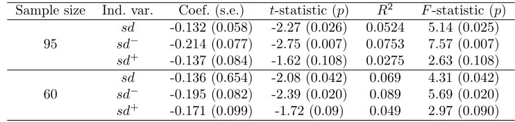
The results are given in Table 1. With respect to the 95 country sample, using the standard deviation
with estimated coefficient -0.132, similar to the Ramey and Ramey (1995) estimate of -0.154 for 92
countries from 1962 to 1985. If the measure of volatility issd−then the estimated coefficient, -0.214,
is significantly larger in absolute magnitude and theR2 fit increases substantially compared to the
sdmeasure. Using the positive semideviation as the regressor provides the smallest fit in terms of
[image:12.612.118.489.236.324.2]R2, and the null hypothesis that the growth rate is independent of sd+ cannot be rejected as the 5% level.
Table 1 Linear regressions of growth rates onsd−,sd+andsdvolatility measures
Sample size Ind. var. Coef. (s.e.) t-statistic (p) R2 F-statistic (p)
sd -0.132 (0.058) -2.27 (0.026) 0.0524 5.14 (0.025) 95 sd− -0.214 (0.077) -2.75 (0.007) 0.0753 7.57 (0.007)
sd+ -0.137 (0.084) -1.62 (0.108) 0.0275 2.63 (0.108)
sd -0.136 (0.654) -2.08 (0.042) 0.069 4.31 (0.042) 60 sd− -0.195 (0.082) -2.39 (0.020) 0.089 5.69 (0.020)
sd+ -0.171 (0.099) -1.72 (0.09) 0.049 2.97 (0.090)
The results for the 60 country 1960-89 sample lead to the same conclusion, and robust regressions
(Huber, 1973) on both samples yield very similar results verifying that they are not the result of
influential outliers. In conclusion, on the basis of these resultssd−is a more appropriate measure of
volatility, and usingsdinstead ofsd−as an explanatory variable greatly underestimates the impact
of volatility upon growth rates.
4 Results
This section investigates the determinants of the three different measures of volatility presented
earlier sd−, sd+ and sd, both for the 1960-89 dataset in Section 4.1 (and a non-OECD country subset in Section 4.4), and for the 1974-89 dataset in Section 4.5. A comparison of the determinants
of the different volatility variables is undertaken in Section 4.2 and the predictive performance on out
of sample observations of the BMA technique is contrasted to other models of volatility in Section
4.3.
4.1 The determinants of downside semideviationsd− in 60 countries (1960-89)
The posterior probabilities of inclusion (or equivalently the posterior probability that the coefficient
variable in explaining volatility. The results of the BMA procedure including the posterior inclusion
probabilities and posterior statistics for the estimated coefficients are given in Table 2. Focusing first
on the downside semideviation measure of volatility the variables whose posterior inclusion
proba-bility is greater than 0.5 are (sign of the posterior mean of the coefficient in brackets): government
consumption share of GDP (+), the trade share of GDP (+), a civil liberties index (+), a degree
of capitalism index(+), the standard deviation of the black market premium (+), the number of
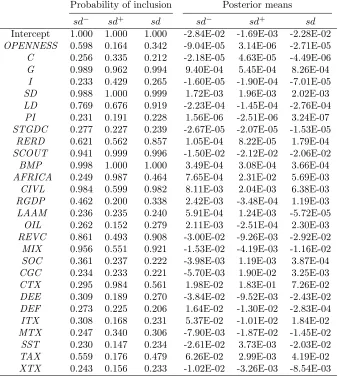
Table 2 Determinants ofsd−,sd+,sdfor a cross-section of 60 countries from 1960-89
Probability of inclusion Posterior means
sd− sd+ sd sd− sd+ sd Intercept 1.000 1.000 1.000 -3.12E-02 -2.10E-02 -3.09E-02
C 0.160 0.990 0.944 3.38E-06 6.57E-05 7.49E-05
G 0.959 0.998 0.992 1.85E-04 2.07E-04 2.69E-04
I 0.266 0.192 0.191 3.77E-05 1.20E-05 2.35E-05
OPENNESS 0.999 0.989 0.997 4.65E-04 3.05E-04 5.35E-04
PRIGHTSB 0.365 0.361 0.281 4.92E-04 -4.68E-04 -2.58E-04
CIVLIBB 0.616 0.802 0.704 1.18E-03 1.56E-03 1.74E-03
RULELAW 0.167 0.146 0.145 -4.52E-04 1.53E-05 1.45E-05
RERD 0.108 0.166 0.129 4.65E-07 -9.88E-07 -2.28E-07
ECORG 1.000 1.000 1.000 4.18E-03 3.39E-03 5.18E-03
BMS 0.905 0.144 0.246 2.61E-05 3.95E-07 4.15E-06
WAR 0.122 0.170 0.139 -6.76E-05 -1.40E-04 -1.39E-04 DEMO 0.256 0.300 0.297 -1.08E-03 -1.03E-03 -1.59E-03 YEARSOPEN 0.172 0.130 0.114 -5.08E-04 4.73E-05 -1.19E-04 ASSASS 0.886 0.620 0.652 -3.05E-03 -1.38E-03 -2.29E-03
BMP 0.994 1.000 1.000 5.48E-03 5.26E-03 9.05E-03
MIX 0.108 0.154 0.134 -4.01E-05 6.32E-05 3.64E-05 OECD 0.441 0.219 0.344 -2.23E-03 -4.54E-04 -1.73E-03
OIL 0.724 0.252 0.306 5.15E-03 8.01E-04 1.84E-03
PI 0.156 0.655 0.497 -2.70E-06 -2.59E-05 -2.52E-05 REVC 0.251 0.151 0.190 1.29E-03 1.15E-04 8.31E-04
RGDP 0.108 0.177 0.141 1.62E-05 4.79E-05 4.06E-05
SCOUT 0.411 0.532 0.331 -1.09E-03 -1.25E-03 -9.15E-04
SOC 0.997 0.999 1.000 1.56E-02 1.39E-02 2.19E-02
STGDC 0.171 0.983 0.912 4.71E-06 8.95E-05 9.55E-05
PINSTAB 0.126 0.140 0.150 4.08E-04 -1.37E-04 -5.86E-04 AFRICA 0.141 0.177 0.154 -2.36E-04 -2.56E-04 -2.68E-04
LAAM 0.661 0.164 0.188 2.96E-03 8.28E-05 3.35E-04
BANK 0.511 0.983 0.983 -8.08E-03 -2.24E-02 -3.25E-02
PRIVATE 0.415 0.613 0.753 4.78E-03 8.23E-03 1.56E-02
PRIVY 0.113 0.393 0.274 5.44E-07 -3.89E-03 -3.07E-03
MONEY 0.153 0.651 0.426 5.03E-04 6.78E-03 5.18E-03
Downside semideviation is found to be positively correlated with government and trade shares
of GDP, implying that economies with a larger government sector and greater degree of openness
suffer from greater volatility. Investment share was found to have a low inclusion probability equal
to 0.266 and the posterior mean is equal to3.77×10−5.
Countries that embrace political rights, civil liberties and rule of law are all found to exhibit
less volatility. It should be noted that because of the high degree of correlation of these three
measures that the BMA procedure often chose only one of these variables. Hence, adding a second
PRIGHTSBhave low posterior inclusion probabilities. The negative relationship between the number
of assassinations per million population and volatility is unexpected.
The economic organization index is higher the more a country favors capitalist forms of
produc-tion and is found to be positively correlated with downside semideviaproduc-tion. At the same time however
the dummy variable for socialist economies is also found to be significant and positive, whereas the
dummy variable for mixed economies is not.
As expected the black market premium and its standard deviation both exacerbate downside
semideviation, and oil producing economies and Latin American economies were all found to exhibit
higher volatility.
Turning to the financial variables the BANK variable is significant and negative leading to the
conclusion that increasing the role of private banks in comparison to central banks in the financial
system leads to lower volatility. This implies that private banks can allocate funds more efficiently
than the central bank. King and Levine (1993) argue that this is because private banks are better
at risk management, information acquisition and creditor monitoring. The probability of inclusion
of the ratio of private domestic assets to total domestic assets (PRIVATE) is quite high 0.415, and
interestingly the greater the degree of financial sophistication as measured by this variable the higher
volatility. This implies that private sector firms use this credit to fund activities that are riskier or
more volatile than a public sector firm would. However, these two variables are quite highly correlated
(ρ= 0.77)and therefore the robustness of these results must be addressed. If multicollinearity is a problem then these estimates should be very sensitive to excluding one of them from the regression,
and should also be sensitive to estimating the model using different subsets of the data.
First, we re-estimate the model two times, each time dropping one of these two variables from the
analysis. IfBANK is excluded, then the probability of inclusion and posterior mean ofPRIVATE are
0.229 and 1.54×10⁻³respectively. Both of these values are less than the associated values for the full regression, however it is important that the sign of the posterior mean is the same, albeit of less
mag-nitude. ExcludingPRIVATE, the relevant estimates forBANK are 0.375 and−4.459×10⁻³, again these are smaller than the estimates of the full model however once again the sign of the posterior
mean does not change. The second method is to impose restrictions on the coefficients of these two
variables thereby eliminating the collinearity. ReplacingBANK and PRIVATE by their difference
(i.e. imposing equal in magnitude but opposite in sign coefficients) leads to an inclusion
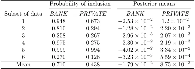
Table 3 Robustness of financial variable effects onsd−for subsets of data
Probability of inclusion Posterior means
Subset of data BANK PRIVATE BANK PRIVATE
1 0.948 0.673 −2.53×10⁻² 1.2×10⁻² 2 0.810 0.294 −1.28×10⁻² 2.20×10⁻³ 3 0.258 0.267 −2.96×10⁻³ 2.07×10⁻³ 4 0.975 0.275 −2.30×10⁻² 2.19×10⁻³ 5 0.999 0.994 −4.02×10⁻² 3.34×10⁻² 6 0.270 0.128 −3.23×10⁻³ 5.59×10⁻⁴ Mean 0.710 0.438 −1.79×10⁻² 8.75×10⁻³
PRIVATE variables with two new interaction variables,BANK×PRIVATE andPRIVATE/BANK, by imposing a multiplicative or inverse interaction between these two variables. The former has an
inclusion probability 0.106 and posterior mean of −1.029×10⁻⁴, whereas the relevant values for the latter variable are 0.623 and 6.106×10⁻³. These restrictions on the coefficients that eliminate the collinearity provide further evidence that higher values ofPRIVATE relative to BANK lead to
higher downside semideviation.
The robustness of the results is also tested by splitting the dataset into 6 subsets of 10 observations
and estimate the model each time excluding one of the subsets. This checks the robustness of the
results not only with respect to collinearity but also with respect to the possibility that outliers are
the main driver of the results. Table 3 provides the probabilities of inclusion and posterior means for
PRIVATE and BANK for each of six subsets of data. The mean probabilities of inclusion are still
high, 0.71 forBANK and 0.438 forPRIVATE, and in all cases the signs of the estimated posterior
means remain unchanged. For the third and sixth subset the probabilities of inclusion are quite
smaller indicating that countries excluded in these two subsets play an important rule in the effect.
Given the high correlation of these two variables it is natural that most of the information will
be embedded within a relatively small number of observations that deviate from the strong linear
correlation found.
These results lead us to believe that the findings of a negative relationship between BANK and
a negative relationship for PRIVATE are not due to multicollinearity and indeterminacy as the
qualitative results survive the exclusion of either variable, various restrictions and transformations,
4.2 Comparison between the determinants of different measures of volatility
A comparison between the variables driving downside and upside semideviation, presented in Table
2, yields some interesting results. In terms of probability of inclusion the most notable differences
are the following. The upside semideviation appears to be driven by the following variables which
are not important in explaining downside semideviation (the sign in brackets denotes the sign of the
derivative of volatility with respect to a variable): consumption share of GDP(+), inflation(−), the standard deviation of the growth of domestic credit (+) and the ratio of liquid liabilities to GDP
(+). Countries with high consumption share of GDP may face greater volatility if consumption is
purchased to a large degree using credit, thereby making it more volatile to interest rate shocks to the
economy. The negative relationship between inflation and upside semideviation is not economically
significant as an increase in one percentage point in inflation leads to a decrease in sd+ by only
−2.59×10⁵, a trivial amount compared to the mean of
sd+
= 0.0148. Also, although the sign of
the relationship between the standard deviation of domestic credit growth is as anticipated it is
interesting that this should not affect downside semideviation. TheBANK variable’s probability of
inclusion increases significant from 0.511 forsd− to 0.983 forsd+,
PRIVATE increases from 0.415
to 0.613 and the ratio of liquid liabilities to GDP (MONEY) from 0.153 to 0.651. Also, note that
the posterior means of these coefficients are much larger in the case ofsd+. The only variable whose inclusion probability falls significantly when analyzing sd+ is the standard deviation of the black market premium.
The determinants of the standard measure of volatility sddiffer from those ofsd− primarily in
terms of a significant effect of consumption share of GDP(+), the standard deviation of the growth
of domestic credit (+) and the higher posterior inclusion probabilities of BANK and PRIVATE
coupled with larger in magnitude posterior means.
4.3 Cross-validation predictive performance of BMA and other models
One of the advantages of BMA is the increase in out of sample predictive performance in comparison
to other methods that do not incorporate model uncertainty. This has been observed for a wide
variety of datasets including predicting growth rates (Fernandez et al, 2001), analyzing infra-red
et al, 1997), in survival analysis (Raftery et al, 1996), in the treatment of primary biliary cirrhosis
of the liver and predicting percent body fat (Hoeting et al, 1999).
The predictive performance of the three different models is compared in Table 4 using the
cross-validation procedure where the dataset is randomly sorted into 6 subsets of 10 data points each.
The models are then estimated on each possible combination of five subsets and used to predict the
observations in the excluded subset. Three sets of predictions were made for each of the dependent
variablessd−
, sd+ and
sdderived from the model with the highest posterior probability (HPP) as
estimated by the BMA procedure, Bayesian predictions from all the models sampled in the BMA
procedure as calculated according to equation 9, and finally predictions from a linear regression
model (LIN) including all the possible covariates.
E( ˆY |Y) =
q
�
k=1
p(Mk|Y)E( ˆY |Mk, Y) (9)
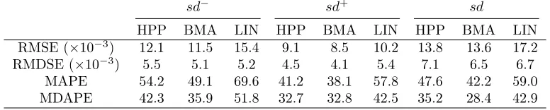
Table 4 presents four different measures of performance, the root mean squared error (RMSE),
the root median squared error (RMDSE), the mean absolute percentage error (MAPE) and finally
the median absolute percentage error (MDAPE). The results in predicting all the volatility variables
are similar, for expositional brevity we discuss those regardingsd−. The BMA predictions were the
most accurate according to all of the performance measures, followed by the model with the highest
posterior probability, and the linear model which performs particularly poorly. It should be noted
that the model with the highest posterior probability can only be derived by performing the BMA
procedure and therefore is not otherwise available to a researcher. The RMSE of the full linear model
predictions is 34 percent higher than that of BMA, and in terms of MAPE it is 42 percent higher or
20.5 percentage points higher. These are extremely large differences that have important economic
significance in forecasting. The median performance measures are all lower than the equivalent mean
performance measures as there is significant positive skew in the errors for each country. Using only
the model with the highest posterior probability instead of all the models visited by the BMA
procedure increases the RMSE by 5.2 percent and the MAPE by 10.2 percent or 5.03 percentage
points. The results are qualitatively similar for the other two measures sd+ andsd, leading to the conclusion that BMA is desirable not only on the grounds of model uncertainty and specification
Table 4 Cross-validation performance of various models in predictingsd−,sd+ andsd
sd− sd+ sd
HPP BMA LIN HPP BMA LIN HPP BMA LIN
RMSE(×10−3
) 12.1 11.5 15.4 9.1 8.5 10.2 13.8 13.6 17.2 RMDSE(×10−3
) 5.5 5.1 5.2 4.5 4.1 5.4 7.1 6.5 6.7
MAPE 54.2 49.1 69.6 41.2 38.1 57.8 47.6 42.2 59.0
MDAPE 42.3 35.9 51.8 32.7 32.8 42.5 35.2 28.4 42.9
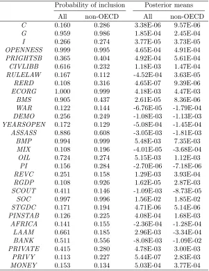
4.4 The determinants ofsd− for non-OECD countries
The validity of the above conclusions with respect to the determinants ofsd− is now examined by
restricting the dataset to non-OECD countries. Table 5 reiterates the results for the full dataset
side by side with the results computed for non-OECD countries for ease of comparison and the
following important differences are noted. The probabilities of inclusion in general do not appear to
be significantly affected with the exception of the probability of inclusion of real GDP per capita
whose probability of inclusion jumps from 0.108 for the full dataset to 0.926 for non-OECD countries,
exhibiting a positive posterior mean. Comparing the posterior means of variables with high inclusion
probabilities for both datasets the black market premium, government share of GDP and BANK
have significantly larger effects onsd− for non-OECD countries.
4.5 The determinants of downside semideviationsd− for 50 countries (1974-89)
The previous analysis did not include variables for government deficits or any debt variables as
these were not widely available from 1960. This dataset includes such variables of particular interest
such as government deficit as a percentage of GDP, long term and short term debt as percentages
of GDP, and GDP shares of various tax revenues (individual, corporate, social security, import
and export tax revenue), full results are presented in Table 6. The debt data is taken from the
Global Development Finance database and the other variables from Levine and Renelt (1992). Since
countries were included on the basis of availability of debt statistics, because debt data was mostly
available for developing countries with relatively low real GDP per capita, this dataset should be
regarded as such. The mean value of RGDP for this dataset is 56.3 percent of the mean value for
the 1960-89 dataset, further statistics are available in Table 11.
The variables determining downside semideviation with posterior probability of inclusion greater
Table 5 Determinants ofsd−for non-OECD countries
Probability of inclusion Posterior means
All non-OECD All non-OECD
C 0.160 0.286 3.38E-06 9.57E-06
G 0.959 0.986 1.85E-04 2.45E-04
I 0.266 0.274 3.77E-05 3.73E-05
OPENNESS 0.999 0.995 4.65E-04 4.91E-04
PRIGHTSB 0.365 0.404 4.92E-04 5.61E-04
CIVLIBB 0.616 0.232 1.18E-03 1.47E-04
RULELAW 0.167 0.112 -4.52E-04 3.63E-05
RERD 0.108 0.316 4.65E-07 9.39E-06
ECORG 1.000 0.999 4.18E-03 4.47E-03
BMS 0.905 0.437 2.61E-05 8.36E-06
WAR 0.122 0.144 -6.76E-05 -1.79E-04
DEMO 0.256 0.249 -1.08E-03 -1.13E-03
YEARSOPEN 0.172 0.129 -5.08E-04 -1.45E-04
ASSASS 0.886 0.608 -3.05E-03 -1.81E-03
BMP 0.994 0.999 5.48E-03 7.35E-03
MIX 0.108 0.196 -4.01E-05 -3.68E-04
OIL 0.724 0.274 5.15E-03 1.12E-03
PI 0.156 0.284 -2.70E-06 -7.18E-06
REVC 0.251 0.158 1.29E-03 3.93E-04
RGDP 0.108 0.926 1.62E-05 2.87E-03
SCOUT 0.411 0.146 -1.09E-03 -8.73E-05
SOC 0.997 0.996 1.56E-02 1.85E-02
STGDC 0.171 0.194 4.71E-06 5.14E-06
PINSTAB 0.126 0.225 4.08E-04 1.68E-03
AFRICA 0.141 0.155 -2.36E-04 -1.28E-04
LAAM 0.661 0.185 2.96E-03 -3.34E-04
BANK 0.511 0.556 -8.08E-03 -1.09E-02
PRIVATE 0.415 0.280 4.78E-03 3.00E-03
PRIVY 0.113 0.227 5.44E-07 2.83E-03
MONEY 0.153 0.134 5.03E-04 3.77E-04
trade share of GDP(−), short term debt as percentages of GDP(+), long term debt as percentages
of GDP(−), real exchange rate distortion(+), a dummy variable for Outward Orientation(−), the
black market premium (+), an index of civil liberties (+), number of revolutions (−), a dummy
variable for Mixed Government (−) and the Ratio of Central Government Tax Revenue to GDP (+).
Comparing the variables with posterior inclusion probability greater than 0.5 that are present
both in the 1974-89 and 1960-89 datasets they are all found to have the same qualitative effect on
sd− with the exception of OPENNESS which is negative for the 1974-89 dataset but positive for
Table 6 Determinants ofsd−,sd+,sdfor a cross-section of 50 countries from 1974-89
Probability of inclusion Posterior means
sd− sd+ sd sd− sd+ sd Intercept 1.000 1.000 1.000 -2.84E-02 -1.69E-03 -2.28E-02 OPENNESS 0.598 0.164 0.342 -9.04E-05 3.14E-06 -2.71E-05 C 0.256 0.335 0.212 -2.18E-05 4.63E-05 -4.49E-06
G 0.989 0.962 0.994 9.40E-04 5.45E-04 8.26E-04
I 0.233 0.429 0.265 -1.60E-05 -1.90E-04 -7.01E-05 SD 0.988 1.000 0.999 1.72E-03 1.96E-03 2.02E-03 LD 0.769 0.676 0.919 -2.23E-04 -1.45E-04 -2.76E-04 PI 0.231 0.191 0.228 1.56E-06 -2.51E-06 3.24E-07 STGDC 0.277 0.227 0.239 -2.67E-05 -2.07E-05 -1.53E-05 RERD 0.621 0.562 0.857 1.05E-04 8.22E-05 1.79E-04 SCOUT 0.941 0.999 0.996 -1.50E-02 -2.12E-02 -2.06E-02 BMP 0.998 1.000 1.000 3.49E-04 3.08E-04 3.66E-04
AFRICA 0.249 0.987 0.464 7.65E-04 2.31E-02 5.69E-03
CIVL 0.984 0.599 0.982 8.11E-03 2.04E-03 6.38E-03 RGDP 0.462 0.200 0.338 2.42E-03 -3.48E-04 1.19E-03 LAAM 0.236 0.235 0.240 5.91E-04 1.24E-03 -5.72E-05 OIL 0.262 0.152 0.279 2.11E-03 -2.51E-04 2.30E-03 REVC 0.861 0.493 0.908 -3.00E-02 -9.26E-03 -2.92E-02 MIX 0.956 0.551 0.921 -1.53E-02 -4.19E-03 -1.16E-02 SOC 0.361 0.237 0.222 -3.98E-03 1.19E-03 3.87E-04 CGC 0.234 0.233 0.221 -5.70E-03 1.90E-02 3.25E-03 CTX 0.295 0.984 0.561 1.98E-02 1.83E-01 7.26E-02 DEE 0.309 0.189 0.270 -3.84E-02 -9.52E-03 -2.43E-02 DEF 0.273 0.225 0.206 1.64E-02 -1.30E-02 -2.83E-04 ITX 0.308 0.168 0.231 5.37E-02 -1.01E-02 1.84E-02 MTX 0.247 0.340 0.306 -7.90E-03 -1.87E-02 -1.45E-02 SST 0.230 0.147 0.234 -2.61E-02 3.73E-03 -2.03E-02 TAX 0.559 0.176 0.479 6.26E-02 2.99E-03 4.19E-02 XTX 0.243 0.156 0.233 -1.02E-02 -3.26E-03 -8.54E-03
of the datasets as the 1974-89 data has only one OECD country and most countries are relatively
poor developing countries. Interestingly,OPENNESS has a negligible, positive impact onsd+as the probability of inclusion is only 0.164 and the posterior mean3.14×10−6.
The ratio of short term debt to GDP is an extremely important determinant (posterior probability
of inclusion=0.988) adversely affectingsd− as it increases. The ratio of long term debt to GDP on
the other hand is found to have a negative relationship withsd−, however the short and long term
debt variables are highly correlated(ρ= 0.79). To ascertain the robustness of these results the BMA model is estimated twice dropping each time one of these debt variables. Including only long term
only the short term debt ratio leads to an inclusion probability of 0.98 with a posterior mean of
1.13×10⁻³ and posterior s.d. of
5.546×10⁻⁴. The results for short term debt are very similar to those found in the original setup including both short and long term debt. Therefore we recommend
accepting the results for short term debt as robust, whereas the effect of long term debt should be
viewed as inconclusive.
From the remaining variables included in this dataset but not in the 1960-89 analysis onlyTAX
has a posterior probability of inclusion greater than 0.5 and is found to be positively related to the
downside semideviation. The relationship of other tax variables withsd− is also positive for
CTX
(corporate) andITX (individual) but negative forXTX (export) andMTX (import), however their
inclusion probabilities are small ranging from 0.247 to 0.308.
Other results worthy of mention include the positive relationship betweenRGDP andsd− with
a relatively high probability of inclusion (0.462). Also, a higher ratio of central government deficit
to GDP was found to increasesd− however the inclusion probability is 0.273.
Comparing the determinants of sd− to those of
sd+ and
sd there are only a few important
qualitative differences. The trade share of GDP exhibits significantly lower probability of inclusion
and is positive forsd+ but remains negative for
sd. Also,CTX now plays an important role as the probability of inclusion is 0.984 and 0.561 forsd+andsdrespectively. At the same time the posterior probability of inclusion ofTAX falls to 0.176 forsd+.
5 Conclusion
This paper’s main contribution to the literature is the application of the Bayesian Model Averaging
technique in examining the determinants of volatility. This technique accounted for the inherent
model uncertainty and permitted a systematic analysis of the robustness of the effects of variables
with respect to the conditioning set of variables. Another innovation is the use of the downside
semideviation of growth rates to more accurately represent the true risk economic agents are
ex-posed to, instead of simply using the standard deviation of growth rates which includes favourable
deviations in growth rates.
Our conclusions regarding the effects of financial variables on volatility deviate in one respect
compared to the literature. Although the ratio of deposit banks domestic assets to deposit banks
argument that financial sophistication and depth lead to lower volatility, the ratio of non-financial,
private domestic assets to total domestic assets was found to be positively related.
The ratio of government expenditure to GDP was consistently found to have a significant positive
relationship with all measures of volatility. Another variable that entered significantly was a measure
of openness, the trade share of GDP, which was positively related to volatility from 1960-89 for a
well balanced dataset of developed and developing countries, whilst exhibiting a less strong negative
relationship for developing countries between 1974-89. As expected, countries that embraced political
rights, civil liberties and rule of law suffered from less volatility. Developing countries exhibited higher
volatility the higher the ratio of short term debt to GDP and the ratio of central government tax
revenue to GDP.
Future research should be directed towards the development and incorporation of panel data
methods into the Bayesian Model Averaging framework, and the requisite collection of sufficiently
broad and accurate time-series data to exploit this.
Acknowledgements The author would like to thank Professor Peng Wang for useful conversations and comments. This research was funded under the Endeavour Cheung Kong Award administered by the
Department of Education, Employment and Workplace Relations of the Australian Government.
References
Acemoglu D, Zilibotti F (1997) Was Prometheus unbound by chance? Risk, diversification, and
growth. Journal of political economy 105(4):709–751
Acemoglu D, Johnson S, Robinson J, Thaicharoen Y (2003) Institutional causes, macroeconomic
symptoms: volatility, crises and growth. Journal of Monetary Economics 50(1):49–123
Aghion P, Banerjee A, Piketty T (1999) Dualism and macroeconomic volatility. Quarterly Journal
of Economics 114(4):1359–1397
Anderson H, Kwark N, Vahid F (1999) Does International Trade Synchronize Business Cycles?
Monash Econometrics and Business Statistics Working Papers
Athanasoulis S, Van Wincoop E (2000) Growth uncertainty and risksharing. Journal of Monetary
Economics 45(3):477–505
Barro R, Lee J (1993) International comparisons of educational attainment. Journal of Monetary
Economics 32(3):363–394
Barro R, Sala-i-Martin X (1995) Economic Growth. New York, NY, McGraw-Hill
Bejan M (2006) Trade openness and output volatility. MPRA Paper 2759
Bekaert G, Harvey C, Lundblad C (2006) Growth volatility and equity market liberalization. Journal
of International Money and Finance 25(3):370–403
Brown P, Vannucci M, Fearn T (1998) Multivariate Bayesian variable selection and prediction.
Journal of the Royal Statistical Society Series B (Statistical Methodology) 60(3):627–641
Buch C, Dopke J, Pierdzioch C (2005) Financial openness and business cycle volatility. Journal of
International Money and Finance 24(5):744–765
Cavallo E (2007) Output Volatility and Openness to Trade: A Reassessment. RES Working Papers
Cecchetti S, Flores-Lagunes A, Krause S (2006) Assessing the sources of changes in the volatility of
real growth. NBER working paper
Clyde M (2009) BAS: Bayesian Adaptive Sampling for Bayesian Model Averaging. R package version
0.45
Clyde M, Desimone H, Parmigiani G (1996) Prediction Via Orthogonalized Model Mixing. Journal
of the American Statistical Association 91(435)
Clyde M, Ghosh J, Littman M (2009) Bayesian adaptive sampling for variable selection and model
averaging. Discussion Paper 2009-16, Duke University Department of Statistical Science
Denizer C, Iyigun M, Owen A (2000) Finance and macroeconomic volatility. World Bank
Di Giovanni J, Levchenko A (2009) Trade openness and volatility. The Review of Economics and
Statistics 91(3):558–585
Easterly W, Islam R, Stiglitz J (2001) Shaken and stirred: Explaining growth volatility. In: Annual
World Bank Conference on Development Economics, pp 191–211
Eicher T, Papageorgiou C, Raftery A (2007) Determining growth determinants: Default priors and
predictive performance in bayesian model averaging. Working Paper no 76, Center for Statistics
and the Social Sciences University of Washington
Fatas A, Mihov I (2001) Government size and automatic stabilizers: International and intranational
evidence. Journal of International Economics 55(1):3–28
Fernandez C, Ley E, Steel M (2001) Model uncertainty in cross-country growth regressions. Journal
Fiaschi D, Lavezzi A (2005) An empirical analysis of growth volatility: A markov chain approach.
http://www-dseecunipiit/persone/docenti/fiaschi/Lavori/growthVolatilitypdf
Frankel J, Rose A (1998) The endogenity of the optimum currency area criteria. The Economic
Journal 108(449):1009–1025
Gastil R (1992) Freedom in the World. Freedom House
Grier K, Tullock G (1989) An empirical analysis of cross-national economic growth, 1951-80. Journal
of Monetary Economics 24(2):259–276
Hakura D (2007) Output Volatility and Large Output Drops in Emerging Market and Developing
Countries. IMF Working Papers 7114(200):1–32
Hall R, Jones C (1996) The Productivity of Nations. NBER Working Papers
Heston A, Summers R, Aten B (2009) Penn world table version 6.3. Center for International
Com-parisons of Production, Income and Prices at the University of Pennsylvania
Hoeting J, Madigan D, Raftery A, Volinsky C (1999) Bayesian model averaging: A tutorial. Statistical
science 14(4):382–401
Huber P (1973) Robust regression: asymptotics, conjectures and Monte Carlo. The Annals of
Statis-tics 1(5):799–821
Kahneman D, Tversky A (1979) Prospect theory: An analysis of decision under risk. Econometrica
47(2):263–291
Kalaitzidakis P, Mamuneas T, Stengos T (2002) Specification and sensitivity analysis of cross-country
growth regressions. Empirical Economics 27(4):645–656
Kent C, Smith K, Holloway J (2005) Declining output volatility: What role for structural change?
In: The changing nature of the business cycle, proceedings of a Conference held at the HC Coombs
Centre for Financial Studies, Kirribilli on, pp 11–12
Kim S (2007) Openness, external risk, and volatility: Implications for the compensation hypothesis.
International Organization 61(01):181–216
King R, Levine R (1993) Finance and growth: Schumpeter might be right. The Quarterly Journal
of Economics 108(3):717–737
Knack S, Keefer P (1995) Institutions and Economic Performance: Cross-country Tests Using
Al-ternative Institutional Measures. Economics and Politics 7:207–227
Kormendi R, Meguire P (1985) Macroeconomic determinants of growth: Cross-country evidence.
Leamer E (1983) Let’s Take the Con out of Econometrics. The American Economic Review 73(1):31–
43
Lensink R, Bo H, Sterken E (1999) Does uncertainty affect economic growth? An empirical analysis.
Review of World Economics 135(3):379–396
Levine R, Renelt D (1992) A sensitivity analysis of cross-country growth regressions. The American
Economic Review 82(4):942–963
Levine R, Loayza N, Beck T (2000) Financial intermediation and growth: Causality and causes.
Journal of monetary Economics 46(1):31–78
Ley E, Steel M (2009) On the effect of prior assumptions in Bayesian model averaging with
appli-cations to growth regression. Journal of Applied Econometrics 24(4):651–674
Liang F, Paulo R, Molina G, Clyde M, Berger J (2008) Mixtures of g Priors for Bayesian Variable
Selection. Journal of the American Statistical Association 103:410–423
Loayza N, Ranciere R, Serven L, Ventura J (2007) Macroeconomic volatility and welfare in developing
countries: An introduction. The World Bank Economic Review 21(3):343
Madigan D, York J, Allard D (1995) Bayesian graphical models for discrete data. International
Statistical Review/Revue Internationale de Statistique pp 215–232
Malik A, Temple J (2009) The geography of output volatility. Journal of Development Economics
90(2):163–178
Markowitz H (1959) Portfolio selection: efficient diversification of investments. John Wiley & Sons
Inc
Martin P, Ann Rogers C (2000) Long-term growth and short-term economic instability. European
Economic Review 44(2):359–381
Mobarak A (2005) Determinants of Volatility and Implications for Economic Development. Review
of Economics and Statistics 87(2):348–361
Montgomery JM, Nyhan B (2010) Bayesian Model Averaging: Theoretical Developments and
Prac-tical Applications. PoliPrac-tical Analysis (Forthcoming)
Van den Noord P (2000) The size and role of automatic fiscal stabilizers in the 1990s and beyond.
OECD Economics Department Working Papers
Posch O (2008) Explaining output volatility: The case of taxation. CESIFO Working Paper No 2751
Raftery A, Madigan D, Volinsky C (1996) Accounting for model uncertainty in survival analysis
Raftery A, Madigan D, Hoeting J (1997) Bayesian model averaging for linear regression models.
Journal of the American Statistical Association 92(437):179–191
Ramey G, Ramey V (1995) Cross-country evidence on the link between volatility and growth. The
American Economic Review pp 1138–1151
Sachs J, Warner A, Åslund A, Fischer S (1995) Economic reform and the process of global integration.
Brookings papers on economic activity 1995(1):1–118
Sala-i-Martin X (1997) I just ran two million regressions. The American Economic Review 87(2):178–
183
Sala-i-Martin X, Doppelhofer G, Miller R (2004) Determinants of long-term growth: a Bayesian
averaging of classical estimates (BACE) approach. The American Economic Review 94(4):813–
835
Ferreira da Silva G (2002) The impact of financial system development on business cycles volatility:
Cross-country evidence. Journal of Macroeconomics 24(2):233–253
Sortino F, Van Der Meer R (1991) Downside risk. The Journal of Portfolio Management 17(4):27–31
Temple J (2000) Growth regressions and what the textbooks don’t tell you. Bulletin of Economic
Research 52(3):181–205
Virén M (2005) Government size and output volatility: Is there a relationship? Research Discussion
Papers, Bank of Finland
Volinsky C, Madigan D, Raftery A, Kronmal R (1997) Bayesian model averaging in proportional
hazard models: Predicting the risk of a stroke. Applied Statistics 46:443–448
Zellner A (1986) On assessing prior distributions and Bayesian regression analysis with g-prior
distributions. Bayesian Inference and Decision Techniques: Essays in Honor of Bruno de Finetti
6:233–243
Zellner A, Siow A (1980) Posterior odds ratios for selected regression hypotheses. In: Bernardo,
DeGroot, Lindley, Smith (eds) Bayesian Statistics: Proceedings of the First International Meeting
held in Valencia (Spain), Valencia: University Press, pp 585–603
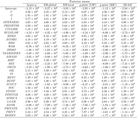
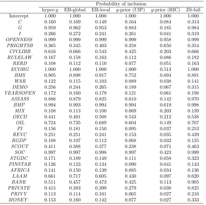
A Robustness of results with respect to different priors
Perhaps the most common criticism of the BMA technique is the dependence on the selection of the prior specification.
Liang et al (2008) investigate the simulated and real performance of the various prior distribution employed also in this
consistency issues that arise with their use, the need to specify the value of the fixed parameter, but also because of
their performance in simulated data which was inferior to that of mixtureg-priors and global- and local-EB priors. To allay any fears with regards the robustness of the results of this paper with respect to the prior specification
we compare results from five different prior specifications: the Unit Information Prior (UIP) which is theg-prior specification whereg=n−1 and the Risk Inflation Criterion (RIC) whereg=k−2, the mixture hyper-gprior using the recommended hyper-parameter value of 3, the EB-global and EB-local prior specification which estimates the
value of g and finally the ZS-full mixture prior. We examine the effects of the prior specification on the two most
important results of this study, the posterior probability of inclusion of variables and their posterior means. Tables 9
and 10 in Appendix B provide the detailed results of modelingsd−with different priors, whilst the similarity of the results are summarized below in Tables 7 and 8 through the Euclidean distance between the relevant estimates and
their correlation.
The posterior probabilities of inclusion are highly correlated (ρ >0.9) for all prior specifications except for the RIC
which still exhibits relatively high correlation (in most cases around 0.7). The lowest Euclidean distances were found
between the EB-global, EB-local and hyper-gspecifications, followed by the UIP and ZS-full priors. The RIC again stands out as being least similar to all the other specifications as the high value ofk2forces the prior probabilities of
[image:28.612.110.491.382.459.2]inclusion of the variables to be very low leading to much lower posterior probabilities of inclusion.
Table 7 Euclidean distance and correlation between posterior probabilities of inclusion for different priors
L2 (ρ) hyper-g EB-global EB-local UIP RIC
EB-global 0.12 (0.998)
EB-local 0.16 (0.997) 0.23 (0.993)
UIP 0.57 (0.975) 0.60 (0.969) 0.46 (0.985)
RIC 1.87 (0.721) 1.88 (0.714) 1.78 (0.748) 1.52 (0.776)
ZS-full 0.70 (0.953) 0.76 (0.942) 0.77 (0.945) 1.08 (0.919) 2.26 (0.628)
Table 8 Euclidean distance and correlation between posterior means for different priors
L2×10−3
(ρ) hyper-g EB-global EB-local UIP RIC
EB-global 2.0 (0.999)
EB-local 1.2 (0.999) 2.6 (0.999)
UIP 3.5 (0.996) 4.6 (0.994) 2.6 (0.998)
RIC 24.3 (0.966) 25.3 (0.967) 23.6 (0.970) 23.2 (0.977)
ZS-full 13.6 (0.950) 14.9 (0.937) 14.1 (0.947) 14.5 (0.944) 30.9 (0.884)
The effects of the prior specification on the posterior means as captured by the correlation coefficient is extremely
robust to all of the tested specifications as in all cases they are greater than 0.88, and in many cases very close to
1 even for the RIC prior. With respect to the Euclidean distance between estimates the ZS-full and RIC priors are
[image:28.612.105.501.522.597.2]