Munich Personal RePEc Archive
Massively parallel computation using
graphics processors with application to
optimal experimentation in dynamic
control
Morozov, Sergei and Mathur, Sudhanshu
Morgan Stanley
10 August 2009
PROCESSORS WITH APPLICATION TO OPTIMAL EXPERIMENTATION IN DYNAMIC CONTROL
SERGEI MOROZOV AND SUDHANSHU MATHUR
Abstract. The rapid growth in the performance of graphics hardware, coupled with re-cent improvements in its programmability has lead to its adoption in many non-graphics applications, including a wide variety of scientific computing fields. At the same time, a number of important dynamic optimal policy problems in economics are athirst of computing power to help overcome dual curses of complexity and dimensionality. We investigate if computational economics may benefit from new tools on a case study of imperfect information dynamic programming problem with learning and experimenta-tion trade-off, that is, a choice between controlling the policy target and learning system parameters. Specifically, we use a model of active learning and control of a linear au-toregression with the unknown slope that appeared in a variety of macroeconomic policy and other contexts. The endogeneity of posterior beliefs makes the problem difficult in that the value function need not be convex and the policy function need not be con-tinuous. This complication makes the problem a suitable target for massively-parallel computation using graphics processors (GPUs). Our findings are cautiously optimistic in that new tools let us easily achieve a factor of 15 performance gain relative to an implementation targeting single-core processors. Further gains up to a factor of 26 are also achievable but lie behind a learning and experimentation barrier of its own. Draw-ing upon experience with CUDA programmDraw-ing architecture and GPUs provides general lessons on how to best exploit future trends in parallel computation in economics. Keywords: Graphics Processing Units·CUDA programming·Dynamic programming· Learning·Experimentation
JEL Classification: C630·C800
1. Introduction
Under pressure to satisfy insatiable demand for high-definition real-time 3D graphics rendering in the PC gaming market, Graphics Processing Units (GPUs) have evolved over the past decade far beyond simple video graphics adapters. Modern GPUs are not single processors but rather are programmable, highly parallel multi-core computing engines with supercomputer-level high performance floating point capability and memory bandwidth. They commonly reach speeds of hundreds of billions of floating point operations per second (GFLOPS) and some contain several billion transistors.
Because GPU technology benefits from large economies of scale in the gaming market, such supercomputers on a plug-in board have become very inexpensive for the raw horse-power they provide. Scientific community realized that this capability could be put to use for general purpose computing. Indeed, many mathematical computations, such as matrix multiplications or random number generation, which are required for complex visual and physics simulations in games are also the same computations prevalent in a wide variety of scientific computing applications from computational fluid dynamics to signal process-ing to cryptography to computational biochemistry. Graphics card manufacturers, such as
Date: April 4, 2011. Version 2.00.
We thank participants of 2009 International Conference on Computing in Economics and Finance and 2010 Econometric Society World Congress for insightful comments. We are grateful to the referee for the valuable suggestions to strengthen the presentation of our results. All remaining errors are our own. The source code for our programs can be retrieved from http://www.wavelet3000.org website.
2 SERGEI MOROZOV AND SUDHANSHU MATHUR
AMD/ATI and NVIDIA, has supported the trend toward general purpose computing by widening the performance edge, by making GPUs more programmable, by including ad-ditional functionality such as single and double precision floating point capability and by releasing software development kits.
The advent of GPUs as a viable tool for general purpose computing parallels the recent shift in the microprocessor industry from maximizing single-core performance to integrating multiple cores to distributed computing (Creel and Goffe,2008). GPUs are remarkable in the level of multi-core integration. For example, high-performance enthusiast GeForce GTX580 GPU from NVIDIA contains 16 multiprocessors each consisting of 32 scalar processor cores, for a total of 512 (NVIDIA,2011). As each scalar processor core is further capable of running multiple threads, it is clear that GPUs represent the level of concurrency today that cannot be found in any other consumer platform. Inevitably, as CPU-based computing is moving in the same massively multi-core (”many-core”) direction, it is time now to rethink algorithms to be aggressively parallel. Otherwise, if a solution is not fast enough, it will never be (Buck, 2005).
Parallel computing in economics is not widespread but does have a fairly long tradi-tion. Chong and Hendry(1986) developed an early parallel Monte Carlo simulation for the econometric evaluation of linear macro-economic models. Coleman(1992) takes advantage of parallel computing to solve discrete-time nonlinear dynamic models expressed as recur-sive systems with an endogenous state variable. Nagurney, Takayama, and Zhang(1995) andNagurney and Zhang(1998) use massively parallel supercomputers to model dynamic systems in spatial price equilibrium problems and traffic problems. Doornik, Hendry, and Shephard(2002) provide simulation-based inference in a stochastic volatility model,Ferrall (2003) optimizes finite mixture models in parallel, while Swann (2002) develops parallel implementation of maximum likelihood estimation. A variety of econometric applications for parallel computation is discussed in Doornik, Shephard, and Hendry (2006). Sims, Waggoner, and Zha (2008) employ grid computing tools to study Bayesian algorithms for inference in large-scale multiple equation Markov-switching models. Tutorial ofCreel and Goffe(2008) urges further application of parallel techniques by economists, whereasCreel (2005) identifies steep learning curve and expensive hardware as the main adoption barriers. None of these studies take advantage of GPU technology.
Financial engineering turned to parallel computing with the emergence of complex deriva-tive pricing models and popular use of Monte-Carlo simulations. Zenios(1999) offers an early synthesis of the evolution of high-performance computing in finance. Later work includes Pflug and Swietanowski(2000) on parallel optimization methods for financial planning un-der uncertainty, Abdelkhalek, Bilas, and Michaelides(2001) on parallelization of portfolio choice,Rahman, Thulasiram, and Thulasiraman(2002) on neural network forecasting stock prices using cluster technology, Kola, Chhabra, Thulasiram, and Thulasiraman (2006) on real-time option valuation, etc. Perhaps due to better funding and more acute needs, quanti-tative analysts on Wall Street trading desks took note of the GPU technology (Bennemann, Beinker, Eggloff, and Guckler,2008) ahead of academic economists.
To the best of our knowledge, ours is one of the first attempts to accelerate economic decision-making computations on graphics chips, alongside a successful demonstration in Aldrich, Fern´andez-Villaverde, Gallant, and Rubio-Ram´ırez(2011) as well as a small number of statistical applications (Tibbits, Haran, and Liechty, 2009; Lee, Yau, Giles, Doucet, and Holmes, 2010). Our application of choice is from a difficult class of imperfect information dynamic programs. In this class, there is an information exploration-exploitation tradeoff, that is, a choice between learning system parameters and controlling the policy target. Specifically, we use a model of active learning and control of a linear autoregression with the unknown slope. The model is a version ofBeck and Wieland’s (2002) Bayesian dual control model that shuts down parameter drift.1 As the system evolves, new data on both sides of the
state evolution equation force revisions of estimates for the location and precision parameters 1Without constant term, our model also could be obtained as a special case of the one studied inMorozov
that characterize posterior beliefs. These evolving beliefs thereby become part of the three-dimensional system state vector to keep track of. The dimension of the state vector matters not only because Bayes rule is nonlinear but, more importantly, because the optimal value function need not be convex, whereas the policy function need not be continuous (Kendrick, 1978; Easley and Kiefer, 1988; Wieland, 2000). Functional approximation methods that rely on smoothness may not work and one is compelled to use brute-force discretization. The endogeneity of information is what makes the problem so complex even when the state dimension is low. This difficulty makes the problem a suitable target for the GPU-based computation.
The most compute-intensive part of the algorithm is a loop updating the value function at all points on a three-dimensional grid. Since these points can be updated independently, the problem can be parallelized easily. For the multi-core CPU-based computation, we use OpenMP compiler directives (Chandra, Menon, Dagum, and Kohr, 2000; Chapman, Jost, and van der Paas, 2007) to generate as many as four threads to run on a state-of-the-art workstation with a quad-core CPU. For the GPU-based computation, we use NVIDIA’s CUDA platform in conjunction with a GeForce GTX280 card supporting this technology. The promise of GPU acceleration is realized as we see initial speedups up to a factor of 15 relative to an optimized CPU implementation. With some additional performance tuning we are able to reach a factor of 26 in some cases.
The paper is laid out as follows. Section2explains the new concepts of GPU programming and available hardware and software resources. Sections3 and4 are dedicated to our case study of the imperfect information dynamic programming problem. The former sets up theoretical background, while the latter contrasts CPU- and GPU-based approaches in terms of program design and performance. Section 5summarizes our findings and offers a vision of what is to come.
2. GPU Programming
2.1. History. Early attempts to harness GPUs for general purpose computing (so called GPGPU) had to express their algorithms using existing graphics application programming interfaces (APIs): OpenGL (Kessenich, Baldwin, and Rost,2006) and DirectX (Bargen and Donnelly,1998). The approach was awkward and thus unpopular.
Over the past decade, graphics cards evolved to become programmable GPUs and on to become fully programmable data-parallel floating-point computing engines. The two largest discrete GPU vendors, AMD/ATI and NVIDIA, have supported this trend by re-leasing software tools to simplify the development of GPGPU applications and adding hard-ware support for programming instructions and higher precision arithmetics to avoid cast-ing computations as graphics operations. In 2006, AMD/ATI released Close-to-the-metal (CTM), a relatively low-level interface for GPU programming that bypasses the graphics API. NVIDIA, also in 2006, took a more high-level approach with its Compute Unified Device Architecture (CUDA) interface library. CUDA extends C programming language to allow the programmer to delegate portions of the code for execution on GPU.2 Although
AMD FireStream technology later included software development kit with higher-level lan-guage support, NVIDIA CUDA ecosystem was the most mature at the inception of our project and was selected as a testbed. Further developments aimed at leveraging many-core coprocessors include OpenCL cross-platform effort (Munshi, Gaster, Mattson, Fung, and Ginsburg, 2011), Intel Ct programming model (Ghuloum, Sprangle, Fang, Wu, and Zhou, 2007), and Microsoft DirectCompute (Boyd and Schmit,2009).3
General purpose computing on GPUs has come a long way since the initial interest in the technology in 2003-2004. On the software side, there are now major applications across the entire spectrum of high performance computing (see, e.g., Hwu (2011) for a recent 2Mathematica natively supports GPU computing via CUDALink, Matlab’s support is in Parallel
Computing Toolbox, while third party wrappers are also available forPython,Fortran,JavaandIDL.
3Heterogeneous cross-vendor device management can be very tedious. SeeKirk and Hwu(2010) for some
4 SERGEI MOROZOV AND SUDHANSHU MATHUR
snapshot), except perhaps computational economics. On the hardware side, many of the original limitations of GPU architectures have been removed and what remains is mostly related to the inherent trade-offs of the massively threaded processors.
2.2. Data Parallel Computing. Until recently, most tools for parallel processing were largely dedicated to task parallel models. The task parallel model is built around the idea that parallelism can be extracted by constructing threads that each have their own goal or task to complete. While most parallel programming is task parallel, there is another form of parallelism that can be exploited.
In contrast to the task parallel model, data parallel programming runs the same block of code on hundreds or even thousands of data points. Whereas typical multi-threaded program to be executed on moderately multi-core/multi-CPU computer handles only a small number of threads (typically no more than 32), a data parallel program to do something like image processing may spawn millions of threads to do the processing on each pixel. The way these threads are actually grouped and handled will depend on both the way the program is written and the hardware the program is running on.
2.3. CUDA Programming. CUDA is one way to implement data parallel programming. CUDA is a general purpose data-parallel computing interface library. It consists of runtime library, set of function libraries, C/C++ development toolkit, extensions to the standard C programming language and a hardware abstraction mechanism that hides GPU hardware from developers. It allows independent and even concurrent execution of both conventional code targeting the host CPU and data parallel code targeting the GPU device. Like OpenMP (Chandra, Menon, Dagum, and Kohr,2000) and unlike MPI (Gropp, Lusk, Skjellum, and Thakur,1999), CUDA adheres to the shared memory model. Furthermore, although CUDA requires writing special code for parallel processing, explicitly managing threads is not re-quired.
CUDA hardware abstraction mechanism exposes a virtual machine consisting of a large number of streaming multi-processors (SMs). A multiprocessor consists of multiple scalar processors (SPs), each capable of executing independent threads. Each multiprocessor has four types of on-chip memory: one set of registers per SP, shared memory, constant read-only memory cache and read-only texture cache.
The main programming concept in CUDA is the notion of a kernel function. A kernel function is a single subroutine that is invoked simultaneously across multiple thread in-stances. Threads are organized into one-, two-, or three-dimensional blocks which in turn are laid out on a two-dimensional grid. Blocks are completely independent of each other, whereas threads within a block are mapped entirely and execute to completion on a single streaming multiprocessor.4 Far more threads can be resident on a multiprocessor than there
are scalar processors. Such over-subscription is the key to hiding memory latencies. If one block stalls waiting on a memory access, another block can proceed, thus keeping the GPU occupied. In order to optimize a CUDA application, one should try to achieve an optimal grid topology in terms of size and number of blocks. More threads in a block reduce the effect of memory latencies, but it will also reduce the number of available registers.
Every block is partitioned into several groups of 32 threads called warps. All threads in the same warp execute the same program. Execution is the most efficient if all threads in a warp execute in lockstep. Otherwise, threads in a warp diverge, i.e., follow different execution paths. If this occurs, the different execution paths have to be serialized leaving some threads idle.
Managing memory hierarchy is another key to high performance. Since there are several kinds of memory available on GPUs with different access times and sizes, the effective bandwidth can vary significantly depending on the access pattern for each type of memory, ordering of the data access, use of buffering to minimize data exchange between CPU and 4A block is a convenient abstraction level in the hierarchy of thread organization, but it does not equate
GPU, overlapping inter-GPU communication with computation, etc. (Kirk and Hwu,2010; NVIDIA, 2011). Memory access to local shared memory including constant and texture memory and well aligned access to global memory are particularly fast. Indeed, ensuring proper memory access can achieve a large fraction of the theoretical peak memory bandwidth which is on the order of 100-200 GB/sec for today’s GPU boards.
The main CUDA process works on a host CPU from where it initializes a GPU, distributes video and system memory, copies constants into video memory, starts several copies of kernel processes on a graphics card, copies results from video memory, frees memory, and shuts down. CUDA-enabled programs can interact with graphics APIs, for example to render data generated in a program.
2.4. CUDA C. CUDA’s extensions to the C programming language are relatively minor. Each function declaration can include a function type qualifier determining whether the function will execute on the CPU or the GPU and if it is a GPU function, whether it is callable from the CPU. Variable declarations also include qualifiers specifying where in the memory hierarchy the variable will reside. Finally, kernels have special thread-identification variables while calls to GPU functions must include an execution configuration specifying grid and thread-block topology and allocations of shared memory on each SM. Functions executed by a GPU have the following limitations: no recursion, no static variables inside functions, no variable number of arguments. Two memory management types are supported: linear memory with pointer access, and CUDA-arrays with access only through texture fetch functions.
Files of the source CUDA C or C++ code are compiled withnvcc, which is just a shell to other tools: cudacc,g++,cl, etc. nvccgenerates: CPU code, which is compiled together with other parts of the application, written in pure C or C++, and special object code targeting a GPU.
2.5. CUDA Fortran. Since there is a vast body of Fortran code in daily use throughout the research community, NVIDIA worked with The Portland Group (PGI) to develop a CUDA Fortran compiler. PGI CUDA Fortran compiler has two usage modes. The first is akin to OpenMP in that it uses accelerator directives to implicitly split portions of the code between CPU and GPU and map loops to automatically use parallel threads. It does not currently include support to automatically control two or more GPUs from the same accelerator region. The second mode is a lower-levelexplicit programming model that allows writing Fortran kernel code, provides language extensions to indicate where a variable or an array is stored and where a subroutine or a function is executed. CUDA Fortran has some advantages over CUDA C since a number of tedious declarations, allocations and data transfers are hidden (The Portland Group, 2010b,a).
In addition to CUDA Fortran, there exist a Fortran-to-CUDA code translator supporting the most commonly used Fortran 95 language constructs, with an exception of input/output statements.
6 SERGEI MOROZOV AND SUDHANSHU MATHUR
in the world (as of November 2010 TOP-500 list), Tianhe-1A, also contains a large number of Tesla GPUs.
2.7. CUDA Resources. As the CUDA development environment is available freely, it is the learning curve that is the steepest adoption barrier. NVIDIA CUDA technology is now being taught at universities around the world, typically in computer science or engineering departments. New textbooks are being written, e.g.,Kirk and Hwu(2010). Numerous sem-inars, tutorials, technical training courses and third-party consulting services are also avail-able to help one get started. Website http://www.nvidia.com/object/cuda education.html collects some of these resources.
3. Case Study: Dynamic programming solution of learning and active experimentation problem
In this section we introduce the imperfect information optimal control problem, dynamic programming approach as well as a couple of useful suboptimal policies.
3.1. Problem Formulation. The decision-maker minimizes a discounted intertemporal cost-to-go function with quadratic per-period losses,
(1) min
{ut}
∞
t=0
E0
"∞ X
t=0
δt (xt−x¯)2+ω(ut−u¯)2
#
,
subject to the evolution law of policy targetxtfrom a class of linear first-order autoregressive
stochastic processes
(2) xt=α+βut+γxt−1+ǫt, ǫt∼ N(0, σ2ǫ).
δ∈[0,1) is the discount factor, ¯xis the stabilization target, ¯uis the ”costless” control,ω≥0 gives relative weight to the deviations ofutfrom ¯u.5 The variance of the shock,σǫ2, is known,
and so are the constant termαand the autoregressive persistence parameter γ ∈(−1,1). Equation (2) is a stylized representation of many macroeconomic policy problems, such as monetary or fiscal stabilization, exchange rate targeting, pricing of government debt, etc.
Only one of the parameters that govern the conditional mean of xt, namely the slope
coefficientβ, is unknown. Initially, prior belief aboutβ is Gaussian:
(3) β∼ N(µ0,Σ0).
Gaussian prior (3) combined with normal likelihood (2) yields Gaussian posterior (Judge, Lee, and Hill,1988), and so at each point in time the belief about unknownβis conditionally normal and is completely characterized by meanµt and variance Σt (sufficient statistics).
Upon observing a realization ofxt, these are updated in accordance with the Bayes law:6
Σt+1=
Σ−t1+
1
σ2 ǫ
u2t
−1
,
µt+1= Σt+1
1
σ2 ǫ
utxt+ Σ−t1µt
.
(4)
Note that the evolution of the variance is completely deterministic.
Under distributional assumptions (2) and (3), the imperfect information problem is trans-formed into a state-space form by defining the extended state containing both physical and informational components:
(5) St= (xt, µt+1,Σt+1)′∈ S ⊆R3.
5Under monetary policy interpretation of the model, ω describes flexibility of monetary policy with
respect to its dual objectives of inflation and output stability (Svensson,1997).
6We use subscriptt+ 1 to denote beliefs afterx
tis realized but before a choice ofut+1is made at the
beginning of periodt+ 1. Technically, it means thatut+1 is measurable with respect to the filtrationFt
As a useful shorthand, encode policy target process (2) and Bayesian updating (4) via mapping
(6) St+1=B(St, xt+1, ut+1).
3.2. Dynamic programming. Our objective is to find the optimal policy functionu∗(S)
that minimizes intertemporal cost-to-go (1) subject to the evolution of the extended state (6), given an initial state S. It is also of interest to compare the value (cost-to-go) of the optimal policy to that of certain simple alternative policy rules. Thus, we will also require computation of the cost-to-go functions of some simple policies.
3.2.1. Inert uninformative policy. So called inert uninformative policy simply sets control impulse to zero, regardless of the current physical statextor the current beliefs. Such policy
is not informative for Bayesian learning in that it leaves the posterior beliefs exactly equal to the prior beliefs. In turn, this allows a closed-form solution for the cost-to-go function corresponding to inert policy:
V0(St) =
(α+γxt−x¯)2−δγ (¯x)2−α2−γx¯(2α−x¯) +γx2t(1 +γ)−2xt(¯x−α+γ2x¯)
(1−δ)(1−γδ)(1−γ2δ)
+ γ
3δ2(x t−x¯)2
(1−δ)(1−γδ)(1−γ2δ)+
σǫ2
(1−δ)(1−γ2δ)+
ω(¯u)2 1−δ .
(7)
Omitting time subscripts, it could be shown that the inert policy cost-to-go function V0
satisfies a recursive relationship:
(8) V0(x, µ,Σ) = (α+γx−x¯)2+ωu¯2+σǫ2+δEV 0(
α+γx+ǫ, µ,Σ).
Relationship (8) can serve as a basis of an iterative computational algorithm, starting from any simple initial guess, for example, Ve0≡0. Upon convergence, the recursive algorithm,
policy iteration in disguise, should approximately recover (7). This provides a simple test of correctness of our CPU-based and GPU-based computations.7
Another use of the inert uninformative policy is to provide explicit bounds on the opti-mal policy with experimentation, u∗
t+1, given the current stateSt, via a simple quadratic
inequality (9)
Et
h
(xt+1−x¯)2+ω u∗t+1−u¯
2i
≤Et
"∞ X
τ=1
δτ−1 (x
t+τ−¯x)2+ω(u∗t+τ−u¯)2
#
≤V0(St).
Asymptotically, the bounds are linear in thexdirection, converge to a positive constant in theµdirection and converge to zero in the Σ direction.
3.2.2. Cautionary myopic policy. Cautionary myopic policy takes account of coefficient un-certainty but disregards losses incurred in periods beyond current. It optimizes the expected one-period-ahead loss function
L(St, ut+1) =
Z
(α+βut+1+γxt+ǫt+1−x¯)2+ω(ut+1−u¯)2
p(β|St)q(ǫt+1)dβdǫt+1
= Σt+1+µ2t+1+ω
u2t+1+ 2 ((µt+1γ)xt−µt+1x¯−ωu¯)ut+1
+ωu¯2+γ2x2t+ ¯x2+σǫ2−2γxx¯ t,
(10)
7Since our numerical implementation restricts the state space to a three-dimensional rectangular cuboid
8 SERGEI MOROZOV AND SUDHANSHU MATHUR
wherep(β|St) andq(ǫt) represent the posterior belief density and the density of state shocks,
respectively. The solution can be found in closed form:
(11) uM Y OPt+1 =−
µγ
Σ +µ2+ωxt+
µ(¯x−α) +ωu¯ Σ +µ2+ω .
Cautionary myopic policy is a useful and popular benchmark in studies of the value of experimentation (Prescott,1972;Easley and Kiefer,1988;Lindoff and Holst,1997;Wieland, 2000; Brezzia and Lai, 2002). From (9), it follows that the myopic policy rule is precisely the mid-point of the explicit bounds on the optimal policy with experimentation. Thus, it is likely to be a good initial guess for the optimization algorithm searching for the actively optimal policy with experimentation, see sections3.2.3and4.1.
The cost-to-go function of the cautionary myopic policy is not explicit but satisfies a recursive functional equation analogous to (8):
VM Y OP(x, µ,Σ) =E α+βuM Y OP(x, µ,Σ) +γx−x¯2+ω(uM Y OP(x, µ,Σ)−u¯)2+σǫ2
+δEVM Y OP α+βuM Y OP(x, µ,Σ) +γx+ǫ, µ′,Σ′,
(12)
where µ′ and Σ′ are the future beliefs given by Bayesian updating (4).8 A method to find an approximate solution of (12) is policy iteration on a discretized state space (i.e., on a grid). The iteration starts with an arbitrary initial guess which is then plugged into the right hand side of (12). Improved guess is obtained upon evaluation of the left hand side at every gridpoint. The process is continued until convergence to an approximate cost-to-go function of the cautionary myopic policy. For a formal justification of the algorithm, see Bertsekas(2005,2001).
3.2.3. Optimal policy with experimentation. Unlike the two previous policies, the optimal policy that takes full account of the value of experimentation is not explicit. It is given by a solution of the Bellman functional equation of dynamic programming,
(13) V(St) = min {ut+1}
L(St, ut+1) +δ
Z
V (St+1)p(β, ǫt+1|St+1)dβdǫt+1
,
where L(St, ut+1) as in (10). Although the stochastic process under control is linear and
the loss function is quadratic, the belief updating equations are non-linear, and hence the dynamic optimization problem is more difficult than problems in the linear quadratic class. FollowingEasley and Kiefer(1988), it could be shown that the Bellman functional operator is a contraction and a stationary optimal policy exists such that the corresponding value function is continuous and satisfies the above Bellman equation. Solution of (13) is a mapping u∗ : S → R from the extended state space to policy choices. Based on above theoretical arguments, an approximate solution can be obtained by the recursive use of discretized version of (13) starting from some initial guess (i.e., value iteration). Upon convergence, one is left with both approximate policy and cost-to-go functions. This process is computationally more demanding than for the earlier two policies due to an additional minimization step.
4. CPU-based versus GPU-based Computations
4.1. CPU-based computation. The approximations to the optimal policy and value func-tion follow the general recursive numerical dynamic programming methods outlined above. Purely for simplicity, we omit several acceleration techniques. In particular, we do not in-troduce alternating approximate policy evaluation steps or asynchronous Gauss-Seidel-type sweeps of the state space (Morozov,2008, 2009a,b). Those are helpful but camouflage the benefits accruing to massively multithreaded implementation.
8It is this nonlinear dynamics of beliefs that precludes closed-form computation of the value function.
Since the integration step in (13) (as well as the integration step implicit in 8 and 12) cannot be carried out analytically, we resort to the Gauss-Hermite quadrature. Further, the actively optimal policy and cost-to-go functions are represented by means of multi-linear interpolation on the non-uniform tensor (Kroneker) product grid in the state space. The non-uniform grid is designed to place grid-points more densely in the high curvature areas, namely in the vicinity of x = ¯x and µ = 0. The grid is uniform along the Σ dimension. Although, in principle, the state space is unbounded, we restricted our attention to a three-dimensional rectangular cuboid. The boundaries were chosen via an apriori simulation experiment to ensure that the high curvature regions are completely covered and that all simulated sequences originating sufficiently deep inside the cuboid remain there for the entire time span of a simulation. The dynamic programming algorithm was iterated to convergence with the relative tolerance9of 1e−6 for the two suboptimal policies and 1e−4 for the optimal policy. Univariate minimization uses a safeguarded multiple restart version of the Brent golden section search (Brent,1973).10
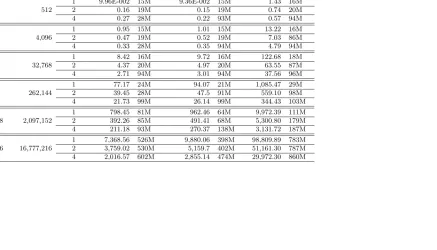
Table1reports runtimes and memory usage of the CPU-based computations for the three types of policies. These were implemented inFortran 90with the outermost loop over the state space explicitly parallelized using OpenMP directives (Chandra, Menon, Dagum, and Kohr, 2000; Chapman, Jost, and van der Paas, 2007). The code was compiled in double precision11with Intel Fortran compiler for 64-bit systems, version 11.0,12and run on a high-end quad-core single CPU workstation utilizing a Core i7 Extreme Edition 965 Nehalem CPU overclocked to 3.4 GHz. In order to reduce the timing noise, the codes were run four times and compute times averaged out for each policy type, CPU thread count and grid size. It should be clear that the deck is intentionally stacked in CPU favor.
Table 1 serves to emphasize very good scaling of the numerical dynamic programming with respect to the thread count, since communication among different threads is not re-quired and workload per thread is fairly uniform. For small grid sizes, the overhead of thread creation and destruction dominates the performance benefit of multiple threads.13 At large grid sizes, memory becomes the limiting factor both in terms of ability to store the cost-to-go function and to quickly update it in memory.
4.2. GPU-based computation. For our GPU-based computations we used a graphics card featuring the GTX280 chip. It has 1.4 billion transistors, theoretical peak performance of 933 Gflops in single precision, peak memory bandwidth of 141.7 Gb/sec and capability to work on 30,720 threads simultaneously. As of early 2009, it was the highest performing consumer GPU available. By the time of publication, it lags significantly behind the GPU performance frontier. For the software stack, we used CUDA version 2.3 for Linux, including the associated runtime, compiler, debugger, profiler and utility libraries.
9Relative tolerance was defined as relative sup norm distance between consecutive approximations
mag-nified by a factor ofδ/(1−δ) based on MacQueen-Porteus bounds (Porteus and Totten,1978;Bertsekas,
2001).
10Preliminary efforts to ensure robustness of the minimization step involved testing our method against
the Nelder-Meade simplex method (Spendley, Hext, and Himsworth,1962;Nelder and Mead,1965;Lagarias, Reeds, Wright, and Wright,1998) with overdispersed multiple starting points (random or deterministic), simulated annealing (Kirkpatrick, Gelatt Jr., and Vecchi,1983;Goffe, Ferrier, and Rogers,1994), direct search (Conn, Gould, and Toint,1997;Lewis and Torczon,2002), genetic algorithm (Goldberg,1989) and their hybrids (Zabinsky,2005;Horst and Paradalos,1994;Paradalos and Romeijn,2002). They all yielded virtually identical results, with occasional small random noise due to the stochastic nature of the search for optimum. On the other hand, these alternative methods, so well suited to nonconvex and nonsmooth problems, required significant computational expense, driven primarily by the sharp increase in the number of function evaluations. Our choice is a compromise between robustness and speed.
11The same code compiled in single precision required more dynamic programming iterations to achieve
convergence to the same tolerance, outweighing the speed benefits of lower precision.
12Intel compilers (Fortran and C) performed significantly better then those from GNU complier collection
(gccandgfortran).
13More elaborate performance-oriented implementation would vary the number of threads depending on
1
0
S
E
R
G
E
I
M
OR
OZ
O
V
A
N
D
S
U
D
H
A
N
S
H
U
M
A
T
H
U
[image:11.612.175.635.134.384.2]R
Table 1. Performance scaling of CPU-based computation under different policies.
Grid size Grid points CPU Threads
Inert Uninformative Myopic Optimal
CPU Time Memory Usage
CPU Time Memory Usage
CPU Time Memory Usage
8x8x8 512
1 9.96E-002 15M 9.36E-002 15M 1.43 16M
2 0.16 19M 0.15 19M 0.74 20M
4 0.27 28M 0.22 93M 0.57 94M
16x16x16 4,096
1 0.95 15M 1.01 15M 13.22 16M
2 0.47 19M 0.52 19M 7.03 86M
4 0.33 28M 0.35 94M 4.79 94M
32x32x32 32,768
1 8.42 16M 9.72 16M 122.68 18M
2 4.37 20M 4.97 20M 63.55 87M
4 2.71 94M 3.01 94M 37.56 96M
64x64x64 262,144
1 77.17 24M 94.07 21M 1,085.47 29M
2 39.45 28M 47.5 91M 559.10 98M
4 21.73 99M 26.14 99M 344.43 103M
128x128x128 2,097,152
1 798.45 81M 962.46 64M 9,972.39 111M 2 392.26 85M 491.41 68M 5,300.80 179M 4 211.18 93M 270.37 138M 3,131.72 187M
256x256x256 16,777,216
GPU-based computation mirrors CPU-based one in all respects except for how it dis-tributes the work across multiple threads. Code fragments below illustrate the differences in the implementation of the main sweep over all points on the grid between the two program-ming frameworks. To focus on the key details, we selected these fragments from a codebase for the evaluation of the cost-to-go function of the cautionary myopic policy. The code for the optimal policy is conceptually similar but is obscured by the details of implementing the minimization operator. We also omit parts of the code that are not interesting, such as checking iteration progress, reading input or generating output files. Omitted segments are marked by points of ellipsis.
Fortran 90 code
1 ...
2 ! set multithreaded OpenMP version using all available CPUs
3 #ifdef _OPENMP
4 call OMP_SET_NUM_THREADS(numthreads)
5 #endif
6 allocate(V(NX,Nmu,NS,2),U(NX,Nmu,NS))
7 ...
8 supval = abs(10.0d0*PolTol+1.0)
9 polit1=0
10 ip = 1
11 ppass =0
12 do while((ip<MaxPolIter+1).and.(ppass.eq.0))
13 ! loop over the grid of the three state variables
14 !$omp parallel default(none) &
15 !$omp shared(NX,Nmu,NS,U,V,X,mu,Sigma,alpha,gamma,delta,omega,ubar,xbar,sigma_eps) &
16 !$omp private(i,j,k)
17 !$omp do
18 do i=1,NX
19 do j=1,Nmu
20 do k=1,NS
21 V(i,j,k,2) = F(U(i,j,k),i,j,k,V)
22 enddo
23 enddo
24 enddo
25 !$omp end do
26 !$omp end parallel
27
28 ! check convergence criterion for the policy function iteration
29 supval = maxval(abs(V(:,:,:,1)-V(:,:,:,2)))
30 checkp = maxval(delta*abs(V(:,:,:,1)-V(:,:,:,2))/((1-delta)*(abs(V(:,:,:,1)))))
31 if (checkp<PolTol) then
32 ppass = 1
33 endif
34
35 ! update the value function
36 V(:,:,:,1) = V(:,:,:,2)
37
38 print *, ’ FINISHED POlICY ITERATION’,ip
39 if (ppass.eq.1) then
40 print *, ’POLICY ITERATION CONVERGED’
41 else
42 print *, ’POLICY ITERATIONS - NO CONVERGENCE’
43 endif
44 ip=ip+1
45 enddo
46 polit1=ip-1
47 ...
The Fortran code is fairly straightforward. The main loop starts on line14and encloses pointwise value updates. So called OpenMPsentinelson lines14-17and25-26tell compiler to generate multiple threads that will execute the loop in parallel. Division of the workload is up to the compiler to decide.
Cuda code (main)
1 ...
2 cudaMalloc((void**) &dX,NX*sizeof(double));
3 ...
4 cudaMemcpy(dX,X,NX*sizeof(double),cudaMemcpyHostToDevice);
5 ...
6 numBlocks=512;
7 numThreadsPerBlock=64;
8 dim3 dimGrid(numBlocks);
12 SERGEI MOROZOV AND SUDHANSHU MATHUR
10
11 // start value iteration cycles
12 supval=fabs(10.0*PolTol+1.0);
13 polit1=0;
14 ip=1;
15 ppass=0;
16 while ((ip<MaxPolIter+1)&&(ppass==0))
17 {
18 // update expected cost-to-go function on the whole grid (in parallel)
19 UpdateExpectedCTG_kernel<<<dimGrid,dimBlock>>>(dU,dX,dmu,dSigma,dV0,drno,dwei,dV1);
20 cudaThreadSynchronize();
21
22 // move the data from device to host to do convergence checks
23 cudaMemcpy(V1,dV1,NX*Nmu*NS*sizeof(double),cudaMemcpyDeviceToHost);
24
25 // check convergence criteria for the policy function iteration if ip>=2
26 ...
27 // update value function, directly on the device
28 cudaMemcpy(dV0,dV1,NX*Nmu*NS*sizeof(double),cudaMemcpyDeviceToDevice);
29 // update value function on host as well
30 cudaMemcpy(V0,V1,NX*Nmu*NS*sizeof(double),cudaMemcpyHostToHost);
31 ...
32 }
33 ...
34 cudaFree(dX);
35 ...
Prior to yet to be released CUDA 4.0, the CUDA code requires separate memory spaces allocated on the host CPU and on the graphics device, with explicit transfers between the two. It replaces the entire loop with a call to a kernel function (line 19). The kernel function is executed by each thread applying a device function to its own chunk of data. The number of threads and their organization into blocks of threads is an important tuning parameter. Having more threads in a block hides memory latencies better but it will also reduce resources available to each thread. For a rough guidance on the tradeoff between size and number of blocks we used NVIDIA’s CUDA occupancy calculator, a handy spreadsheet tool. Even though NVIDIA recommends the number of threads per block that is a multiple of available streaming multiprocessors (30 for GTX280), we were restricted to the powers of two by our implementation of divide-and-conquer algorithm for on-device reduction (see section4.4). Additionally, all the model parameters as well as fixed quantities such as grid sizes or convergence tolerances were placed in constant memory to facilitatelocal access to these values by each thread. No further optimizations were initially applied. The final code snippet shows some internals of the kernel code but omits the device function. Internals of the device function are functionally identical to similar Fortran code and perform the Gauss-Hermite integration of the trilinearly interpolated value function.
CUDA kernel code
1 ...
2 __device__ inline double UpdateExpectedCTG(double u,double x,double mu,double Sigma,
3 double alpha, double gamma, double delta, double omega, double sigma_eps,
4 double xbar, double ubar, int NX,int Nmu, int NS, int NGH, double* XGrid,
5 double* muGrid, double* SigmaGrid, double* V, double* rno, double* wei);
6 __global__ void UpdateExpectedCTG_kernel(double* U,double* X,double* mu,
7 double* Sigma,double* V0,double* rno,double* wei,double* V1)
8 {
9
10 //Thread index
11 const int tid = blockDim.x * blockIdx.x + threadIdx.x;
12 const int NUM_ITERATION= dc_NX*dc_Nmu*dc_NSigma;
13 int ix,jmu,kSigma;
14
15 //Total number of threads in execution grid
16 const int THREAD_N = blockDim.x * gridDim.x;
17
18 //ech thread works on as many points as needed to update the whole array
19 for (int i=tid;i<NUM_ITERATION;i+=THREAD_N)
20 {
21 //update expected cost-to-go point-by-point
22 ix=i/(dc_NSigma*dc_Nmu);
23 jmu=(i-ix*dc_Nmu*dc_NSigma)/dc_NSigma;
25 V1[i]=UpdateExpectedCTG(U[i],X[ix],mu[jmu],Sigma[kSigma],dc_alpha,
26 dc_gamma,dc_delta,dc_omega,dc_sigmasq_epsilon,dc_xstar,dc_ustar,
27 dc_NX,dc_Nmu,dc_NSigma,dc_NGH,X,mu,Sigma,V0,rno,wei);
28 }
29 30 }
31 ...
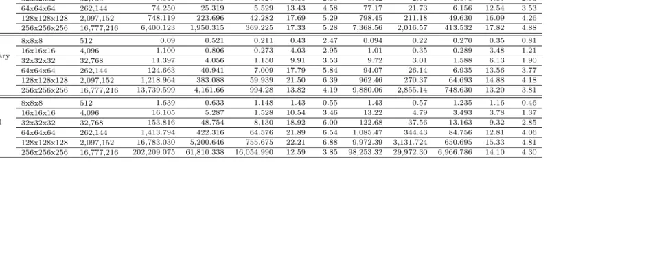
4.3. Speed comparison. Table 2 documents initial timing results for GPU implementa-tions in single and double precision in comparison to single-threaded and multi-threaded CPU-based implementations. These are done for all three policies and across a range of grid sizes. As with CPU-based implementation, CUDA codes were timed repeatedly to reduce measurement noise.14
Several things are worth noticing in table 2. First, for the small problem sizes, multi-threading is actually detrimental to performance due to the fixed costs of thread management and memory allocation. CPU threads are more ”heavy-weight”, requiring larger thread creation/destruction overheads, with four CPU cores finishing slower than one core in several cases. Second, across all cases, GPU wins over single CPU in 86% of cases, and over four cores in 94% of cases, only loosing for the smallest grid sizes. Third, the margin of victory is oftentimes quite substantial, in some more than factor of 20. Fourth, single precision calculation on the GPU is generally faster than double precision, especially taking into consideration that the dynamic programming algorithm takes up to 50% more iterations to converge in single precision, with the exact ratio depending on grid size and policy type. In contrast, the speed of single precision calculation on the CPU is only marginally different from double precision, after accounting for the convergence effect. This is because GPUs have separate units dedicated to double and single precision floating point calculations but CPUs do not. Moreover, consumer versions of NVIDIA GPUs have only a fraction of resources devoted to double precision compared to single precision.15 With this in mind, it is actually surprising how little difference there is between the double and single precision results on GPU. This is likely due to the underutilization of the floating point resources in either case.
To provide a uniform basis for the comparison we transformed the timing results for the double precision case reported in table2 into gridpoints per second speeds. The speeds are plotted in figure1against the overall size of the grid, in semi-log space. For all three policy types, performance of the single-threaded code tends to fade with the problem size, most likely due to memory limitations. In contrast, the performance of the two- and four-threaded versions of the two suboptimal policies initially improves with the problem size as fixed costs of multiple threads are spread over a longer runtime but starts to fall relatively early. The more complex calculation per grid point for the optimal policy causes a downward trend in the performance throughout the entire grid size range. The GPU performance, on the other hand, continues to improve until moderately large grid size but still drops for the very large grids.
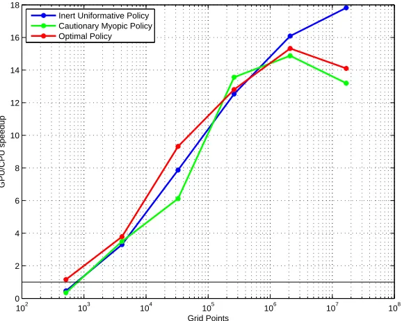
Figure 2 distills performance numbers further by focusing on the GPU speedup ratio relative to the single CPU. It emphasizes two things – somewhat limited applicability of the GPU speedups and a substantial speed boost for moderately sized grids even for double precision.16 Beyond the optimal problem size, the gain in speed tapers off.17
14The GPU runs have remarkably lower variability of measured runtime compared to the CPU-based
runs, possibly due to less intervention from the operating system.
15Only the recent models in NVIDIA’s Tesla line of GPUs that is targeted for high-performance
comput-ing instead of gamcomput-ing improve substantially on the ratio of double precision and scomput-ingle precision capabilities.
16Similar but slightly slower results were reported in an earlier working paper version using CUDA 2.2,
except for largest grids where computational acceleration faltered precipitously.
17Additionally, if the same GPU is used simultaneously to drive a graphic display, GPU threads are
1
4
S
E
R
G
E
I
M
OR
OZ
O
V
A
N
D
S
U
D
H
A
N
S
H
U
M
A
T
H
U
[image:15.612.127.677.160.357.2]R
Table 2. Runtime comparison of CPU and baseline GPU-based calculations.
Policy Grid size Grid Points
Single Precision Double Precision
CPU1 CPU4 GPU CPU1GPU CPU4GPU CPU1 CPU4 GPU CPU1GPU CPU4GPU
Inert
Uninfor-mative Policy
8x8x8 512 0.114 0.723 0.231 0.49 3.13 0.096 0.27 0.216 0.46 1.25
16x16x16 4,096 0.735 0.689 0.261 2.82 2.64 0.95 0.33 0.288 3.30 1.15
32x32x32 32,768 7.039 2.669 1.027 6.85 2.60 8.42 2.71 1.070 7.87 2.53
64x64x64 262,144 74.250 25.319 5.529 13.43 4.58 77.17 21.73 6.156 12.54 3.53
128x128x128 2,097,152 748.119 223.696 42.282 17.69 5.29 798.45 211.18 49.630 16.09 4.26 256x256x256 16,777,216 6,400.123 1,950.315 369.225 17.33 5.28 7,368.56 2,016.57 413.532 17.82 4.88
Cautionary Myopic
Policy
8x8x8 512 0.09 0.521 0.211 0.43 2.47 0.094 0.22 0.270 0.35 0.81
16x16x16 4,096 1.100 0.806 0.273 4.03 2.95 1.01 0.35 0.289 3.48 1.21
32x32x32 32,768 11.397 4.056 1.150 9.91 3.53 9.72 3.01 1.588 6.13 1.90
64x64x64 262,144 124.663 40.941 7.009 17.79 5.84 94.07 26.14 6.935 13.56 3.77
128x128x128 2,097,152 1,218.964 383.088 59.939 21.50 6.39 962.46 270.37 64.693 14.88 4.18 256x256x256 16,777,216 13,739.599 4,161.66 994.28 13.82 4.19 9,880.06 2,855.14 748.630 13.20 3.81
Optimal Policy
8x8x8 512 1.639 0.633 1.148 1.43 0.55 1.43 0.57 1.235 1.16 0.46
16x16x16 4,096 16.105 5.287 1.528 10.54 3.46 13.22 4.79 3.493 3.78 1.37
32x32x32 32,768 153.816 48.754 8.130 18.92 6.00 122.68 37.56 13.163 9.32 2.85
102 103 104 105 106 107 108 0
2 4 6x 10
4
Grid points
Grid points per second
Inert Uniformative Policy
1 CPU 2 CPU 4 CPU GPU
102 103 104 105 106 107 108
0 1 2 3 4x 10
4
Grid points
Grid points per second
Cautionary Myopic Policy
1 CPU 2 CPU 4 CPU GPU
102 103 104 105 106 107 108
0 1000 2000 3000 4000
Grid points
Grid points per second
Optimal Policy
[image:16.612.161.454.82.317.2]1 CPU 2 CPU 4 CPU GPU
Figure 1. Speed comparison of CPU and GPU-based approaches for dou-ble precision calculations.
102 103 104 105 106 107 108
0 2 4 6 8 10 12 14 16 18
Grid Points
GPU/CPU speedup
Inert Uniformative Policy Cautionary Myopic Policy Optimal Policy
Figure 2. Ratio of GPU and single CPU speeds for double precision cal-culations.
4.4. Code Tuning. The substantial speed gains demonstrated above are a testament to the potential of throughput-oriented GPU architecture and resulted from a straightforward
[image:16.612.163.452.373.604.2]16 SERGEI MOROZOV AND SUDHANSHU MATHUR
code translation. Whether our initial implementation leaves additional performance on the table is the focus of this section.
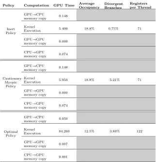
[image:17.612.144.466.173.507.2]To identify potential performance bottlenecks of the initial implementation we made use of the CUDA profiler tool. Results for the 64x64x64 problem configuration are reported in table3.18
Table 3. CUDA Profiler report based on runs with 64x64x64 grid size.
Policy Computation GPU Time Average Occupancy
Divergent Branches
Registers per Thread
Inert Policy
GPU→CPU
memory copy 0.148
Kernel
Execution 5.400 18.8% 0.75% 71
GPU→GPU
memory copy 0.000
CPU→GPU
memory copy 0.074
Cautionary Myopic
Policy
GPU→CPU
memory copy 0.148
Kernel
Execution 5.950 18.8% 5.21% 71
GPU→GPU
memory copy 0.000
CPU→GPU
memory copy 0.074
Optimal Policy
GPU→CPU
memory copy 0.050
Kernel
Execution 84.260 12.5% 3.83% 122
GPU→GPU
memory copy 0.007
CPU→GPU
memory copy 0.001
Ostensibly, the execution time is dominated by the kernel computations while explicit transfers between various memory spaces account for less than 3% of the time. This is helpful since memory accesses are normally much slower than computations. Also favorable to the performance is a low incidence of divergent branches. Divergent branches refer to the situations when different threads within the same group of threads called warp take different paths following a branch condition. Thread divergence leads to performance degradation.
On the other hand, average occupancy seems low. Average occupancy indicates that only 10-20% of threads (out of possible 30,720) can be launched simultaneously with enough per-thread resources. While high occupancy does not necessarily equal performance, low occupancy kernels are not as adept at hiding latency. NVIDIA recommends average latency of 25% or higher to hide the memory latency completely (NVIDIA, 2009c). The limiting factor to occupancy is the number of registers, the fastest type of on-chip memory used to store intermediate calculations. More registers per thread will generally increase the performance of individual GPU threads. However, because thread registers are allocated from a global register pool, the more registers are allocated per thread will also reduce the
18Slight discrepancy in runtimes between tables2and3is due to a small variation between the individual
maximum thread block size, thereby reducing the amount of thread parallelism (NVIDIA, 2009c). NVIDIA CUDA compiler provides a switch that allows control of the maximal number of registers per thread. If this option is not specified, no maximum is assumed. In addition, for a given register limit, occupancy may be tuned by manipulating the execution configuration, i.e., the number of thread blocks and the block size. For simplicity, we fixed execution configuration parameters at values suggested by the CUDA occupancy calculator. To assess the impact of specifying different maximal amount of registers per thread, we recompiled and rerun the code for the actively optimal control using register values from 20 to 128. 20 is the smallest amount that allows the program to run, and 128 is the maximum allowed by the GT200 architecture. The results of that experiment, in terms of grid points per second, are shown in figure3for several problem sizes. The best results for each problem size are marked with solid circles and also collected in table4.19
0 20 40 60 80 100 120
102 103 104
Register Maximum
Gridpoints per second
[image:18.612.163.450.236.466.2]8x8x8 16x16x16 32x32x32 64x64x64 128x128x128 256x256x256
Figure 3. Register use and GPU speeds for active optimal policy calculation.
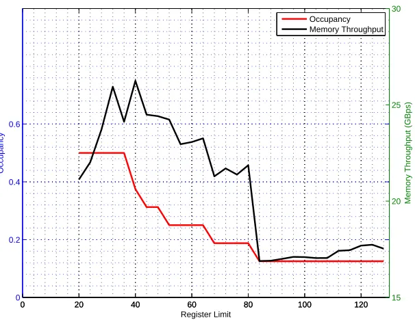
The good news in figure 3and table 4is an ability to extract additional 40% of perfor-mance. The bad news is that tuning register use is not automatic but labor intensive. It also appears to be problem size specific. For the smallest problems it is best to use almost all registers, while for medium-size problems it is enough to restrict register usage to 32 – 48 range. The largest problems again favor large number of registers. As scarcity of registers limits the amount of thread parallelism, this explains hump-shaped performance curve in figure2. Since occupancy is in an inverse relationship with register use, the optimal occu-pancy exhibits inverse U shape with respect to the problem size. That occuoccu-pancy is not equal performance is upheld in figure 4. Occupancy declines throughout the entire range of register use limits, and yet the optimal register use is achieved in the interior. Still, the greatest performance boost is achieved for problem sizes with the largest difference between the baseline and the optimized occupancy values.
Comparison of figures 3 and 4 suggests a very strong correlation of performance and memory throughput reported by CUDA profiler. It makes sense based on the following considerations.
Each thread in our implementation sequentially applies Bellman updates to one or more point on the state-space grid (more than one if the total grid size exceeds the number of
18 SERGEI MOROZOV AND SUDHANSHU MATHUR
Table 4. Speedup due to register tuning for active optimal policy calculation.
Problem size
Default solu-tion time
Optimal register restriction
Register-optimal solution time
Speedup factor
Optimal occu-pancy
8x8x8 1.253 124 1.241 0.95% 12.5%
16x16x16 3.493 92 3.291 6.14% 12.5%
32x32x32 13.163 32 9.273 41.95% 50%
64x64x64 84.756 40 58.961 43.75% 37.5%
128x128x128 650.695 48 578.393 12.50% 31.25%
256x256x256 6,966.786 120 6,966.982 0.00% 12.5%
0 20 40 60 80 100 120
0 0.2 0.4 0.6
Occupancy
Register Limit
0 20 40 60 80 100 120 15
20 25 30
Memory Throughput (GBps)
[image:19.612.156.459.381.615.2]Occupancy Memory Throughput
Figure 4. Occupancy and memory throughput against register use for active optimal policy calculation for 64x64x64 problem size.
memory.20,21For each such value, the kernel performs four floating point operations, result-ing incompute to global memory access ratio(CGMA) of about 4. Low CGMA ratio means that memory access is indeed the limiting factor (Kirk and Hwu, 2010).
Since the reported memory throughput falls short of the advertised theoretical maximum of 141.6 GB/sec, there are additional factors hindering performance. These factors have to do withlocalityof memory accesses. Indeed, the 256 values of the cost-to-go function needed to update a given point could be widely spread out in the state space since they depend on the magnitude of control impulse under consideration. Therefore, the Gauss-Hermite integration inside the value function update induces a memory access pattern that is not random but somewhat irregular in that large and variable control impulse effectively spreads out integration nodes further apart so that access to more distant grid indices is required.22 Since the memory access is irregular, a popular strategy of storing subvolumes of the state space in constant memory will not work (Kirk and Hwu, 2010). Improving memory access requires more sophisticated approaches. One such approach is to do with textures.
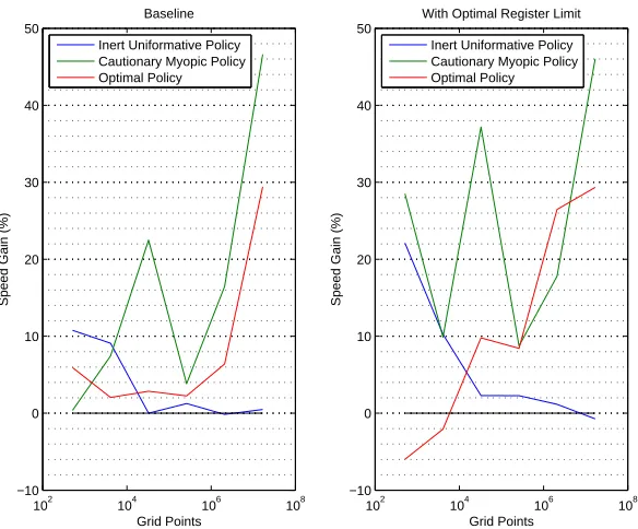
Due to their graphics heritage, GPUs have dedicated hardware to process and store textures which can be thought of as two-dimensional “skin” to be mapped onto a surface of a three-dimensional object. Formally, a texture can be any region in linear memory which is read-only and cached, potentially exhibiting higher bandwidth if there is 3D locality in how it is accessed. Textures are read from kernels using device functions calledtexture fetches.23 Due to the special memory layout of texture fetches, the codes with random or irregular memory access patterns typically benefit from binding multi-dimensional arrays to textures instead of storing them in the global on-device memory. Thus, texture fetches can provide higher memory bandwidth to computational kernels.24 With this in mind, we bound our policy and value arrays to one-dimensional textures and used texture fetches inside CUDA kernel. Results are shown in figure 5 for baseline case with unlimited per-thread registers in the left panel and for register-tuned case in the right panel.
The inert uninformative policy features a regular access pattern to the one-dimensional arrays storing value and policy function approximations. Thus, it does not benefit much from texture memory access. Under cautionary myopic policy, using textures can be highly beneficial, especially for larger problem sizes. Calculations for the optimal policy are also consistently accelerated by texture fetches for larger problems, but for smaller problems it could lead to a performance loss.
An important performance recommendation, according to NVIDIA(2009c), is to mini-mize data transfers between the host and the device because those transfers have much lower bandwidth than internal device data transfers. In our initial implementation, convergence check was done on the CPU which necessitated transfer of data out of the GPU device. A convergence check amounts to calculating the maximum difference between two arrays, and is thus areduction (Kirk and Hwu,2010). Reduction step could be performed on the GPU. We extended our computational kernel to accommodate on-device partial reduction in which each thread block computes the maximal absolute difference for the array indices assigned to it. This is done by traversing a comparison tree in a way that aligns memory
20Technically, our algorithm featuresgathermemory access type.
21Potentially, not all of these grid points are distinct, in which case there is a loss of efficiency due to
repeated yet unnecessary memory access. Adapting the code to track repetitions requires each thread to locally store potentially large number of values thus increasing register pressure and complicating code flow. For these two reasons we decided against access tracking.
22Do-nothing policy is an exception since it leaves beliefs and integration nodes unchanged. 23Texture fetches are not available in CUDAFortran.
24In addition, texture fetches are further capable of hardware-accelerated fast low-precision trilinear
20 SERGEI MOROZOV AND SUDHANSHU MATHUR
102 104 106 108
−10 0 10 20 30 40 50
Grid Points
Speed Gain (%)
Baseline
Inert Uniformative Policy Cautionary Myopic Policy Optimal Policy
102 104 106 108
−10 0 10 20 30 40 50
Grid Points
Speed Gain (%)
With Optimal Register Limit
[image:21.612.161.453.80.322.2]Inert Uniformative Policy Cautionary Myopic Policy Optimal Policy
Figure 5. Speed gains due to accessing memory via textures.
accesses by each thread, unrolls loops and uses shared memory. This partial reduction code was derived fromHarris(2005). It has high-performance on large arrays but is rather com-plex and repetitive, especially for the optimal policy calculations which are hampered by CUDA’s restriction on function pointers preventing us from splitting the optimization code into a separate function. Once the first thread in a thread block finds the max norm dis-tance between successive value function approximations for the slice assigned to that thread block, the second round of reduction commences where a small subset of threads is used to compute the largest of thread block maxima. This step is short since there could be no more than 512 thread blocks. For simplicity, we have not taken up a suggestion byBoyer, Tarjan, Acton, and Skadron(2009) to reorder reduction and computation steps to eliminate wasteful synchronization barrier between first and second rounds.
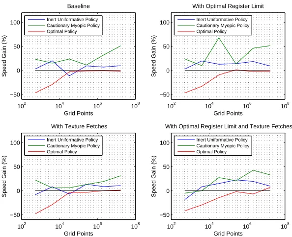
Figure6summarizes the performance impact due to on-device reduction in combination with other methods. On-device reduction is not always beneficial, especially for small prob-lem sizes as well as for more complex algorithms. For example, optimal policy computation is accelerated only in combination with other techniques and for the largest problem sizes, since it is largely compute-bound, not communication-bound. On the other hand, comput-ing the value of the cautionary myopic policy profits from on-device reduction practically across the board. In combination with register tuning, it can gain impressive 68%. The speed gain tends to diminish when on-device reduction is in addition to texture fetches since both techniques aim to alleviate the same memory bottleneck.
CUDA offers several additional techniques and tools that may help performance in some applications. These include page-locked memory (pinned memory) mapped for access by GPU for higher transfer speeds and eligibility for asynchronous memory transfers as well as atomic functions that are guaranteed to be performed without interference from other threads. We investigated these techniques and found neither speed advantage nor disadvan-tage for our code.
102 104 106 108 −50
0 50 100
Grid Points
Speed Gain (%)
Baseline
Inert Uniformative Policy Cautionary Myopic Policy Optimal Policy
102 104 106 108
−50 0 50 100
Grid Points
Speed Gain (%)
With Optimal Register Limit
Inert Uniformative Policy Cautionary Myopic Policy Optimal Policy
102 104 106 108
−50 0 50 100
Grid Points
Speed Gain (%)
With Texture Fetches
Inert Uniformative Policy Cautionary Myopic Policy Optimal Policy
102 104 106 108
−50 0 50 100
Grid Points
Speed Gain (%)
With Optimal Register Limit and Texture Fetches
[image:22.612.157.454.80.322.2]Inert Uniformative Policy Cautionary Myopic Policy Optimal Policy
Figure 6. Speed gains due to on-device partial reduction.
a search over multiple performance dimensions. It is doubtful that researchers will have enough time on their hands to do much beyond simple tune-ups.
For the smallest problem sizes, GPU computing is not worth the effort and can be even counterproductive.
Our best case speedups seem to fall behind the speedups up to 500 fold reported in Aldrich, Fern´andez-Villaverde, Gallant, and Rubio-Ram´ırez(2011), the first application of the GPU computing technology to solving dynamic equilibrium problems in economics. There are several reasons for the discrepancy. First and foremost, the largest speedup in Aldrich, Fern´andez-Villaverde, Gallant, and Rubio-Ram´ırez (2011) is achieved when the GPU and the CPU rundifferent algorithms that implement a binary search. The CPU ver-sion exploited the monotonicity of the value function to place state-dependent constraints on the control variable, while the GPU version ignored those constraints as they created depen-dencies that were not parallelizable. To the extent that both approaches yielded accurate solutions, handicapping the CPU version is clearly not necessary. In contrast, our com-parison used exactly the same algorithm in both versions. More generally, we concur with with a defensive argument made by Intel software engineers (Lee, Kim, Chhugani, Deisher, Kim, Nguyen, Satish, Smelyanskiy, Chennupaty, Hammarlund, Singhal, and Dubey,2010) that stunningly large (in excess of 100 fold) speedups are more likely reflective of an in-ferior CPU algorithm than of a superior GPU implementation. For a fair comparison, both CPU and GPU implementations need to be fine-tuned, a potentially difficult task in both cases. Second, memory requirements of the dynamic program in Aldrich, Fern´ andez-Villaverde, Gallant, and Rubio-Ram´ırez (2011) are very light, since the state-space grid is one-dimensional.25 This means more computational work done per one memory access.
25We disagree withAldrich, Fern´andez-Villaverde, Gallant, and Rubio-Ram´ırez’s (2011) argument that
22 SERGEI MOROZOV AND SUDHANSHU MATHUR
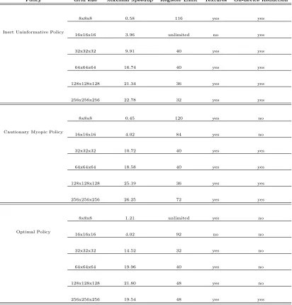
Table 5. Maximal speedups.
Policy Grid size Maximal Speedup Register Limit Textures On-device Reduction
Inert Uninformative Policy
8x8x8 0.58 116 yes yes
16x16x16 3.96 unlimited no yes
32x32x32 9.91 40 yes yes
64x64x64 16.74 40 yes yes
128x128x128 21.34 36 yes yes
256x256x256 22.78 32 yes yes
Cautionary Myopic Policy
8x8x8 0.45 120 yes no
16x16x16 4.02 84 yes no
32x32x32 10.72 40 yes yes
64x64x64 18.58 40 yes yes
128x128x128 25.19 36 yes yes
256x256x256 26.25 72 yes yes
Optimal Policy
8x8x8 1.21 unlimited yes no
16x16x16 4.02 92 no no
32x32x32 14.52 32 yes no
64x64x64 19.96 40 yes no
128x128x128 21.80 48 yes no
256x256x256 19.54 48 yes yes
Since memory access is slower than the speed of arithmetic operations,Aldrich, Fern´ andez-Villaverde, Gallant, and Rubio-Ram´ırez(2011) face less severe memory bottleneck. Third, we skew the results in the CPU favor by using faster overclocked CPU, and higher performing Intel Fortran compiler.26
5. Concluding Remarks
This paper offers a qualified endorsement of data parallel massively multi-threaded com-putation using CUDA for comcom-putational economics. With relatively little effort, we were able to boost performance by a factor of about 15 relative to an optimized single-thread
in parallel with computation between memory locations with different access proximity will be of serious concern for high-dimensional dynamic equilibrium problems that economists may attempt to solve.
CPU implementation. During our project’s lifetime, the performance leading edge moved significantly to further GPU advantage. By the time of publication, new graphics cards and CUDA driver updates more than quadrupled the performance of our code, a faster ramp compared with the increase in CPU core count and frequency over the same period.27
We expect that with the subsequent NVIDIA GPU generations, code-named ”Kepler” and ”Maxwell”, the performance ramp will be extended further.
Nevertheless, attaining the full potential of the graphics hardware proved more involved as we needed to know certain details of how the underlying architecture actually works. Notably, one has to heed the management of the thread hierarchy by balancing size and number of blocks, by hiding memory latency through overlapping inter-GPU communica-tion with computacommunica-tion, by explicitly optimizing memory access patterns across different memory types and different memory locations. Appropriate combinations of performance tuning techniques, which essentially trade one resource constraint for another, can make a huge difference in the final performance. Plausible strategies to optimize around various performance gating factors embrace ideas of maximizing independent parallelism; work-load partitioning and tiling; loop unrolling; using shared, constant and texture memories; data prefetch; asynchronous data transfers and optimizing thread granularity (seeNVIDIA (2009c)). Since in different applications, different resource limits may be binding, perfor-mance tuning is prone to dull guess work.28
The tedium of debugging parallel code can detract from GPU programming. Parallel code begets new breed of errors including resource contention, race conditions and deadlocks. Since even very unlikely event will likely occur given sufficiently many trials, the severity of these errors rapidly escalates with the number of parallel threads. For example, triggering a subtle synchronization bug may be extremely unlikely with a small number of concurrent threads, but the same bug will have a much higher probability of manifestation in a parallel program with tens of thousands of threads. Even so, uncovering and solving a bug in a parallel program will not necessarily get easier with higher likelihood of bug’s appearance. This is because effective reasoning about parallel workflow is difficult even for seasoned programmers. Fortunately, with each new iteration of CUDA development tools it gets easier to visualize parallel workflow and debug code. Reusing tested code further reduces novice errors and performance barriers. NVIDIA supports code reuse by providing templated algorithms and data structures inThrustand NPPlibraries as well as by extending the set of implemented C++ features.29
GPU-based numerical libraries are in their infancy as well. While basic linear algebra, some signal processing (e.g., FFT) and elementary random number generation are covered (NVIDIA, 2009a; Tomov, Dongarra, Volkov, and Demmel, 2009; NVIDIA, 2010, 2009b; Howes and Thomas,2007), important areas such as multivariate optimization and quadra-ture are not. Integration with different programming languages such as Fortran or Java or with computing environments such asMatlaborMathematicais also incomplete.
Development of parallel computing on GPUs is bound to have an impact on high per-formance computing industry as graphics cards are already inexpensive and ubiquitous. Indeed, with peak performance of nearly one teraflop, the compute power of today’s graph-ics processors dwarfs that of the commodity CPUs while costing only a few hundred dollars. If nothing else, emergence of GPU as a viable competitor to traditional CPU for high per-formance computing will elicit a response by the major CPU manufacturers, a duopoly of Intel and AMD. Even though CPU development may appear glacial compared to quantum performance leaps in GPUs, nothing prevents CPUs from adopting ideas of data parallel processing. CPUs are growing to have more cores, capable of more threads, add special 27Initial experiments with GTX580 graphics card reduced the longest runtimes for the optimal policy
calculation by a factor of 6 compared with GTX280.
28Kirk and Hwu(2010) report in one their case studies that exhaustive search over various tuning
param-eters and code organizations resulted in 20% larger performance increase than was available by exploiting heuristic considerations.
29For example, version 4 of CUDA toolkit includes support for virtual functions and dynamic memory