Survey of Methods of Solving TSP along with its Implementation using Dynamic Programming Approach

Survey of Methods of Solving TSP along with its

Implementation using Dynamic Programming Approach

Chetan Chauhan

SSSIST SEHORE India

Ravindra Gupta

SSSIST Sehore India

Kshitij Pathak

MIT Ujjain India

ABSTRACT

The Traveling salesperson problem is one of the problem in mathematics and computer science which haddrown attention as it is easy to understand and difficult to solve. In this paper, we survey the various methods/techniques available to solve traveling salesman problem and analyze it to make critical evaluation of their time complexities. An implementation of the traveling salesman problem using dynamic programming is also presented in this paper which generates optimal answer and tested with 25 cities and it executes in reasonable time.

Keywords

Traveling Salesman problem, Heuristic approach, Dynamic Programming, Greedy Method, Exact Solution Approaches

1.

INTRODUCTION

Traveling Salesman Problem (TSP) is classical and most widely studied problem in Combinatorial Optimization [1]. It has been studied intensively in both Operations Research and Computer Science since 1950s as a result of which a large number of techniques were developed to solve this problem. Much of the work on TSP is not motivated by direct applications, but rather by the fact that it provides an ideal platform for study of general methods that can be applied to a wide range of Discrete Optimization Problems. Indeed, numerous direct applications of TSP bring life to research area and help to direct future work. The idea of problem is to find shortest route of salesman starting from a given city, visiting n cities only once and finally arriving at origin city. TSP is represented by complete edge-weighted graph G=(V,E) with V being set of n=|V| nodes or vertices representing cities and EV×V being set of directed edges or arcs. Each arc (i,

j)E is assigned value of length dijwhich is distance between cities i and j with i, jV . TSP can be either asymmetric or symmetric in nature. In case of asymmetric TSP, distance between pair of nodes i, j is dependent on direction of traversing edge or arc i.e. there is at least one arc(i, j) for which dij≠dji. In symmetric TSP, dij=djiholds for all arcs in E.

The goal in TSP is thus to find minimum length Hamiltonian Circuit [2]of graph, where Hamiltonian Circuit is a closed path visiting each of n nodes of G exactly once. Thus, an optimal solution to TSP is permutation π of node indices {1,...,n} such that length f(π) is minimal, where f(π)is given

by,

( ) ∑

2.

HISTORY

The origin of the TSP and its name is somewhat obscure. It appears to have been discussed informally among mathematicians for many years. Surprisingly little in the way of results has appeared in the mathematical literature. One of the first appearances of tours and circuits in the mathematical

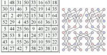
literature is in a 1757 paper by the great Leonard Euler. The paper concerns a solution of the knight’s tour problem in chess, that is, the problem of finding a sequence of knight’s moves that will take the piece from a starting square on a chessboard, through every other square exactly once and returning to the start. Euler’s solution is depicted in Fig 1, where the order of moves is indicated by the numbers on the squares [4].

Fig 1: Knight’s tour

An Irish mathematician sir W. R. Hamilton and the English mathematician T. P. Kirkman already treated mathematical problems related to the TSP in the 1800’s [5].

The German handbook from 1832 by B.F. Voigt goes through 47 German cities(fig 2) and is actually of very good quality and might even be optimal given the travel conditions of that time[6].

Fig 2: The Commis-Voyageur tour for 47 Germancities

In 1859 Sir William Hamilton contributed to the growth of graph theory by inventing the Icosiangame (or Hamilton’s aroundthe world problem) (fig 3) that requires a playerto complete a tour using only specified connectors through 20 points [7].

Volume 52– No.4, August 2012

ending point is the same as the starting point [8], a game which clearly is not far away from the TSP formulation. The objective is to go around the world by passing through each city once and only once. The solution is called a “Hamilton cycle” (fig 4). Sir Hamilton got into serious financial difficulties trying to market his game [9].

Fig 3: The Icosian Game

Fig4: Dodecahedron

The general form of the TSP appears to have been first studied by mathematicians during the 1930s in Vienna and at Harvard, notably by Karl Menger, who defines the problem, considers the obvious brute-force algorithm, and observes the non-optimality of the nearest neighbour heuristic.

Shortly after this the TSP became popular among mathematicians at Princeton University. There does not exist any authoritative source for the origin of the problems name, but according to Merrill Flood and A.W. Tucker it became introduced by its present day name in 1934 as part of a seminar given by HasslerWhitney at Princeton University [10].

Merrill Flood (Columbia University), as early as 1937, tried to obtain near optimal solutions in reference to routing of school buses. Both Flood and A.W. Tucker (Princeton University) recall that they first heard about the problem in a seminar talk by Hassler Whitney at Princeton in 1934, who is credited with naming the traveling salesman problem. In the 1950s and 1960s, the problem became increasingly popular in scientific circles in Europe and the USA. California experts, George Dantzig, Delbert Ray Fulkerson and Selmer M. Johnson, were part of an exceptionally strong and influential center for thenew field of mathematical programming, housed at the RAND Corporation in Santa Monica. They expressed TSP as an integer linear program and developed the cutting plane method for its solution. Using these new methods they took up the computational challenge of TSP, solving a 49-city instance by hand to optimality by constructing a tour and proving that no other tour could be shorter. Along the way

they set the stage for the study of integer programming. In the following decades, the problem was studied by many researchers from mathematics, computer science, chemistry, physics, and other sciences. [11]

In 1972 Richard M. Karp showed that the problem of finding a Hamiltonian cycle was complete, which implies the NP-hardness of TSP. This supplied a scientific explanation for the apparent computational difficulty of finding optimal tours.

In 1962, the TSP became publicly known to a great extent in the USA due to a contest by Procter & Gamble consisting of a problem instance of 33 cities. The $ 10 000 Price for the shortest solution was at that time enough to purchase a new house in many parts of the country (fig 5).

Fig5: The 33 city contest from 1962.

In 1970, Held and Karp developed a one-tree (A tree containing exactly one cycle) relaxation which provides a lower bound within 1 % from the optimal. It achieves this by relaxing the degree constraints using a Minimum Spanning Tree (MST) and Lagrangian multipliers.

In 1972, Karp proved the NP-completeness of the Hamiltonian Cycle Problem (HCP) from which the NP-completeness of the TSP follows almost directly [12].

In 1973, Lin and Kernighan proposed a variable-depth edge exchanging heuristic for refining an initial tour. The method, now known as the “Lin-Kernighan” algorithm, performs variable k-opt moves that allow intermediate tours to be longer than the original tour. A k-opt move can be seen as the removal of k edges from a TSP tour followed by the patching of the resulting paths into a tour using k other edges .

In 1976, Christofides published a tour construction method, that achieves a 3/2-approximation [i.e. guaranteeing a solution no worse than 3/2 times the optimal solution] by using a MST and “Perfect Matching”. Apart from the euclidean TSP this is still the tightest approximation ratio known [13].

[15], which is one of the first publications discussing “Neural Network” algorithms. Both articles use the TSP as a working example.

In 1990, Bentley developed a new highly efficient variant of the k-d tree [a binary search tree structure extended in k dimensions] data structure, which is used for proximity checking, while he was working on heuristics for the TSP [16].

In 1991, Reinelt composed and published TSPLIB [17], a library containing many of the test problems studied over the last 50 years [18].

In 1992, David Applegate, Robert Bixby, VašekChvátal and William Cook solved a 3038 TSP city instance to optimality using the exact TSP solver program Concorde, on which they started the development in 1990. Concorde has ever since been involved in all proven optimality tour records.

In 1996, the first Polynomial Time Approximation Scheme (PTAS) for the euclidean TSP was devised by Arora. The PTAS finds tours with length (1 + ) times the optimal and has a running-time of nO( 1/ ). Since it had previously been proven that both the general as well as the Metric Traveling Salesman Problem (MTSP) do not have a PTAS this result was received with surprise.

In 1998 KeldHelsgaun released a highly efficient and improved extension of the Lin-Kernighan heuristic algorithm, called Lin-Kernighan- Helsgaun (LKH). Among other characteristics it uses one-tree approximations for determining candidate edge-lists (10a list containing the preferred routes between two cities) and 5-opt moves. LKH has later been extended and it has participated with Concorde in solving the largest instances of the TSP to this day. Furthermore LKH has been holding the record for the 1 904 711 city World TSP Tour11 since 2003. It has subsequently improved the tour three times (most recently in May 2010). Table 1 shows the short history of Travelling Salesman Problem.

Table 1Short History of the TSP [22]

Year Milestone Contributors

1954

49-point instance solved by LP and by

adding cutting planes manually.

Dantzig, Fulkerson and Johnson

1970

Lagrangian relaxation. Error about 1%.

Held and Karp

1973 k-Opt heuristic. 1% to

2% above optimal. Lin and Kernighan

1976 1:5-approximation. Christodes

1983 Simulated annealing-based heuristic.

Kirkpatrick, Gelatt and Vecchi

1985

Recurrent neural network-based heuristic.

Hopfield and Tank

1992 TSP heuristics by

using k-d trees. Bentley

1995

7,392-point instance solved by LP and cutting

planes generation (Concorde).

Applegate, Bixby, Chv_atal and Cook

1996

PTAS for the Euclidean TSP. nO(1/ϵ) time.

Arora

1998

Improved k-opt heuristic (LKH). Within

1% above optimal.

Helsgaun

2004

24,978-point instance solved by LKH and proved by Concorde.

Applegate, Bixby, Chvatal, Cook and Helsgaun

2006 85,900-point instance solved by Concorde.

Applegate, Bixby, Chvatal, Cook, Espinoza, Goycoolea and Helsgaun

3.

TSP SOLVER

3.1Exact Solvers

There are two groups of exact solvers. One of these is solving relaxations of the TSP Linear Programming formulation and uses methods like Cutting Plane, Interior Point, Branch-and-Bound and Branch-and-Cut. Another smaller group is using Dynamic Programming. For both groups the main characteristic is a guarantee of finding optimal solutions at the expense of running time and space requirements.

3.1.1

Branch and Bound

Branch and bound was discovered independently by at least three groups. Firstly Dantzig et al. [19] applied the method to the ATSP. This extremely significant paper also introduced several other innovations. A more general description was provided by Land and Doig [20] in the context of solving integer programming problems by linear programming. Finally, the approach was described and named branch and bound by Little et al. [21] in an application to the TSP. The Branch and Bound method implicitly enumerates all the feasible solutions, using calculations where the integer constraints of the problems are relaxed. In other words the branch and bound strategy divides a problem to be solved into a number of sub-problems. It is a system for solving a sequence of sub-problems each of which may have multiple possible solutions and where the solution chosen for one problem may affect the possible solutions of later sub-problems. To avoid the complete calculation of all partial trees, we first try to find a practical solution and note its value as an upper bound for the optimum. As the distance exceeds the distance of the upper bound the calculations are done. If a new cheaper solution was found, its value is used as the new upper bound. This method is convenient for 40 to 60 nodes (cities).

3.1.2

The Cutting Plane

The groundbreaking work of Dantzig, Fulkerson, and Johnson [23] on the traveling salesman problem introduced the cutting-plane method, which can be used to attack any problem minimizecT x subject to x  S; (1)

where S is a finite subset of some Euclidean space IRm, provided that an efficient algorithm to recognize points of S is available. This method is iterative; each of its iterations begins with a linear programming relaxation of (1), meaning a problem

minimizecT _{x subject to Ax≤b; (2)}

Volume 52– No.4, August 2012

belongs to S, then it constitutes an optimal solution of (1); otherwise, some linear inequality separates x* from S in the sense of being satisfied by all the points in S and violated by x*; such an inequality is called a cutting plane or simply a cut.

3.1.3 Branch and Cut

A primitive version of this idea was already applied to theTSP by Hong (1972) and Miliotis (1976).Grotschel, Junger&Reinelt (1984) applied it to the so-calledLinear Ordering Problem.The term branch-and-cut was coined by Padberg&Rinaldi(1987, 1991).They used it to solve very large TSP instances (up to 2000cities or so).

The branch and cut method solves the linear program without the integer constraint using the regular simplex algorithm. When an optimal solution is obtained, and this solution has a non-integer value for a variable that is supposed to be integer, a cutting plane algorithm is used to find additional linear constraints which are satisfied by all feasible integer points but violated by the current fractional solution. If such an inequality is found, it is added to the formulation, such that resolving it will yield a different solution which is hopefully "less fractional". This process is repeated until either an integer solution is found (which is then known to be optimal) or until no more cutting planes are found. We may normally end with an optimal solution however, in practice we may not have an exact separation algorithm and it may return no violated inequality although there are some. If we have not terminated with an optimal solution to IP, we branch. We decompose the problem into two new problems, i.e., adding upper and lower bounds to a variable whose current value is fractional. The problem is split into two versions, one with the additional constraint that the original variable is greater than or equal to the next integer greater than the intermediate result, and one where this variable is less than or equal to the next lesser integer. Then we solve each new problem recursively by the same method and the optimal solution to the original problem will bethe better of these two solutions. Such an integration of enumeration with cutting plane is the core of the branch and cut method. This method has been successful in finding optimal solutions of large instances of a closely related problem, the Symmetric Traveling Salesman Problem (STSP). However, compare to TSP, the amount of research carries out on branch and cut applied to CVRP is still quite limited. Similar to in branch and bound algorithms, the central problem of branch and cut is that the tree generated by the branching procedure becomes too large and termination seems unlikely within a reasonable amount of time.

3.1.4 Dynamic Programming

It is a technique for efficiently computing recurrences by storing partial results and re-using them when needed.It is well known that dynamic-programming recursions can be expressed as shortest-path problems in a layered network whose nodes correspond to the states of the dynamic program. Accordingly, the method proposed in Balas (1996) associates with a TSP satisfying , a network G* := (V *;A*) with n + 1 layers of nodes, one layer for each position in the tour, with the home city (city 1) appearing at both the beginning and the end of the tour, hence both as source node s (the only node in layer 1) and sink node t (the only node in layer n+1) of the network. The structure of G*, to be outlined below, is such as to create a one-to-one correspondence between tours in G satisfying condition (to be termed feasible) and s−t paths in G*. Furthermore, optimal tours in G correspond to shortest s − t paths in G*.

3.1.5 Brute-force method.

When one thinks of solving TSP, the first method that might come to mind is a brute-force method. The brute-force method is to simply generate all possible tours and compute their distances. The shortest tour is thus the optimal tour.

3.2

Non-exact Solvers

These solvers offer potentially non-optimal but typically faster solutions. In a way the opposite trade-off of the exact solvers. Non-exact solvers can be subdivided into:

Approximation Algorithms These algorithms come with a worst case approximation factor for the found solution. The two traditional methods for solving the TSP are a pure MST based algorithm, which achieves a factor 2 approximation and a combined MST and Minimum Matching Problem (MMP) based algorithm due to Christofides, which achieves a factor 3/2 approximation. Both methods are restricted to the MTSP as they depend on the triangle inequality. The PTAS for Euclidean TSP is mainly a theoretical result due to its prohibitive running time.

Heuristic Algorithms These algorithms only promise a feasible solution. They range from simple tour-construction methods like Nearest Neighbour, Clarke-Wright and Multiple Fragment1 to more complicated tour improving algorithms like Tabu Search and Lin-Kernighan. Finally there is a group of fascinating algorithms which unfortunately tend to combine approximate solutions and large running-times. Here we find methods like Simulated Annealing, Genetic Algorithms, Ant Colony Algorithms and machine learning algorithms like Neural Networks.

3.2.1 Christofides’ Algorithm

The goal of the Christofides algorithm (named after NicosChristofides) is to find a solution to the instances of the traveling salesman problem where the edge weights satisfy the triangle inequality. Let G(V, w) be an instance of TSP, i.e. G is a complete graph on the set V of vertices with weight function w assigning a nonnegative real weight to every edge of G.[24]

It works by first constructing a minimum spanning tree T for the set ofcities, and then a minimum length matching M is done on the vertexes with odd degree inT. Combining M with

T gives us a connected graph where every vertex has an evendegree, this graph now holds an Euler tour [25] i.e. a cycle that passes through each edgeexactly once. By first identifying the Euler tour, the TSP tour is then created bytraversing the Euler tour.

3.2.2 Clarke-Wright Algorithm

The Clarke-Wright savings heuristic (Clarke-Wright or simply CW for short) is derived from a more general vehicle routing algorithm due to Clarke and Wright [1964]. In terms of the TSP, we start with a pseudo-tour in which an arbitrarily chosen city is the hub and the salesman returns to the hub after each visit to another city. (In other words, we start with a multigraph in which every non-hub vertex is connected by two edges to the hub). For each pair of non-hub cities, let the

TSP with n cities is in O(n2 log(n)) with a space complexity in O(n2 _{) [26].}

3.2.3 NearestNeighbour

This method is a natural strategy for the TSP, because it mimics the way the traveling salesman selects a travel route. It selects a starting point and then always selects the nearest city to be added to the tour, it then “walks” to that city and repeats by choosing a new non-selected city, until all cities is in the tour. To complete the tour, an edge is added between the last selected city and the starting city. A general version of this heuristic has running time of Θ(N2

) [27]. However, if the distnce metric satisfies the triangle inequality, then the best guarantee, in terms of tour quality, is NN(I)/OPT(I) ≤ (0. 5)(

log2N + 1 ). However, Rosenkrantz et al. [28] found instances for which the ratio grows as Θ(logN).

3.2.4 Insertion Heuristics

Insertion heuristics are quite straight forward, and there are many variants to choose from. The basics of insertion heuristics is to start with a tour of a subset of all cities, and then inserting the rest by some heuristic. The initial subtour is often a triangle or the convex hull. One can also start with a single edge as subtour.

Reinelt [29] lists nine insertion heuristics. Most have run time O(n2 ) with two variants having run time O(n2 log(n)). The initial path typically consists of between 0 and 2 vertices.

3.2.5 The Greedy Heuristic

The greedy heuristic constructs a tour iteratively, by inserting an edge of lowest cost into a set T, consistent with the requirement to eventually result in a tour. The arrangement is given in Algorithm .Reinelt [30] reports a proof by Frieze that where the triangular inequality holds, the greedy heuristic is ratio bound by log(n).

To solve TSP using Greedy Approach, we look at all the arcs coming out of the city (node) and choose the n cheapest arcs. If those n cheapest arcs forms a Hamiltonian cycle than we have an optimal solution.

This algorithm can be implemented with running time Θ(N2logN). As you may have noticed, this algorithm is slower than the nearest neighbor algorithm. Like the nearest neighbor algorithm, it can be shown that for all instances satisfying triangle inequality, worst-case tour quality is Greedy(I)/OPT (I) ≤ (0.5)( log2N + 1) however, the worst examples known for Greedy only make the ratio grow as (log N)/( 3 log logN) [31].

The Greedy algorithm normally keeps within 15-20% of the Held-Karp lower bound [32]

3.2.6 Gutin and Yeo Algorithm

More recently Gutin and Yeo [33] have provided an approximation heuristic they term the greedy expectation heuristic. The authors provide details for both the ATSP and quadratic assignment problems.

For the ATSP, the algorithm operates by recursively constructing a tour. The algorithm starts with an empty tour and a complete directed graph K. At each step in the process an edge, e, is selected from the incumbent K such that the average cost of tours containing e is minimised. This edge is added to the partially completed tour. The recursion repeats with a modified K (excluding e and certain associated edges). It terminates when a complete tour is constructed.

3.2.7 Hill Climbing (HC)

In computer science, hill climbing is a mathematical optimization technique which belongs to the family of local search. It is an iterative algorithm that starts with an arbitrary solution to a problem, then attempts to find a better solution by incrementally changing a single element of the solution. If the change produces a better solution, an incremental change is made to the new solution, repeating until no further improvements can be found[34].

3.2.8 Lin-Kernighan

The Lin-Kernighan (LK) algorithm [35] is generally considered to be one of the mosteffective methods for generating optimal or near-optimal solutions for the TSP.However, the design and implementation of LK is not simple. There are many designsand implementation decisions to be made, and most decisions have great influence on theperformance. The creation of the LK was inspired by the observation that a static K in theK-Opt method is not necessary the best solution. Designers wanted to use a different K-Optin different stages in the execution of the heuristic. In practice it has been shown thatit is difficult to know what K to use to achieve the best compromise between running time and quality of the solution [3]. Lin and Kernighan removed this drawback by introducinga powerful variable-Opt algorithm. The algorithm changes the value of K

during its execution [3].

3.2.9 The Metropolis Algorithm

In its original form, the Metropolis algorithm simulates the behaviour of systems governed by statistical mechanics [36]. In the context of optimization, the algorithm is similar to iterative improvement, but utilizes two stochastic mechanisms. These mechanisms allow local minima to be escaped [37].

3.2.10 Simulated Annealing (SA)

Simulated annealing is a well-known meta-heuristic search method that has been used successfully in solving many combinatorial optimization problems. It is a hill climbing algorithm with the added ability to escape from local optima in the search space. However, although it yields excellent solutions, it is very slow compared to a simple hill climbing procedure.

The term simulated annealing is adopted from the annealing of solids, where we try to minimize the energy of the system using slow cooling until the atoms reach a stable state. The slow cooling technique allows atoms of the metal to line themselves up and to form a regular crystalline structure that has high density and low energy. The initial temperature and the rate at which the temperature is reduced is called the annealing schedule.

The theoretical foundation of SA was led by Kirkpatrick et al.

in 1983 [38], where they applied the Metropolis algorithm

Volume 52– No.4, August 2012

displacement is accepted with a certain probability exp(−E/kbT) where E is the change in energy resulting from the displacement, T is the current temperature, and kb is a constant called a Boltzmann constant . Depending on the value returned by this probability either the new displacement is accepted or the old state is retained. For any given T, a sufficient number of iterations always leads to thermal equilibrium. The SA algorithm has also been shown to possess a formal proof of convergence using the theory of

Markov Chains [40].

3.2.11 Tabu Search (TS)

Glover in 1977 [41]. Since then, it has been widely used for solving combinatorial optimization problems. Its name is derived from the word ‘taboo’ meaning forbidden or restricted. The central feature of the approach is the use of memory in the search in the process. At the simplest level, tabu search operates much like interactive improvement, but with additional restrictions on which solutions in the neighborhood of some solution s may be visited. At the conceptual level, the restrictions are enforced by maintenance of a set of tabu solutions, T . These are only moved to if there is good reason to do so, with the decision to explore these dependent on the aspiration criterion. At the practical level, the tabu set is maintained as a combination of previously visited moves, a history set, and/or set of rules governing which moves are valid given the current solution, its neighborhood and the history set.

3.2.12 Ant Colony Optimization (ACO)

Ant Colony Optimization is a meta-heuristic technique that is inspired by the behavior of real ants. Its principles were established by Dorigoet al. in 1991 [42]. Real ants cooperate to find food resources by laying a trail of a chemical substance called ‘pheromone’ along the path from the nest to the food source. Depending on the amount of pheromone available on a path, new ants are encouraged, with a high probability, to follow the same path, resulting in even more pheromone being placed on this path. Shorter routes to food sources have higher amounts of pheromone. Thus, over time, the majority of ants are directed to use the shortest path. This type of indirect communication is called ‘stigmergy’ [43], in which the concept of positive feedback is exploited to find the best possible path, based on the experience of previous ants.

3.2.13 Genetic Algorithms (GAs)

The idea of simulation of biological evolution and the natural selection of organisms dates back to the 1950’s. One of the early pioneers in this area was Alex Fraser with his research published in 1957 [44,45]. Nevertheless, the theoretical foundation of GAs were established by John Holland in 1975 [46], after which GAs became popular as an intelligent optimization technique that may be adopted for solving many difficult problems.

The theme of a GA is to simulate the processes of biological evolution, natural selection and survival of the fittest in living organisms. In nature, individuals compete for the resources of the environment, and they also compete in selecting mates for reproduction. Individuals who are better or fitter in terms of their genetic traits survive to breed and produce offspring. Their offspring carry their parents’ basic genetic material, which leads to their survival and breeding. Over many generations, this favorable genetic material propagates to an increasing number of individuals. The combination of good characteristics from different ancestors can sometimes produce ‘super fit’ offspring who out-perform their parents. In

this way, species evolve to become better suited to their environment.

4.

PROPOSED SOLUTION

This paper implements a Dynamic Programming method for finding an optimal solution to the traveling salesman problem.This method givescorrectresult in reasonable time. The dynamic programming method proceeds as follows.

Traveling salesman problem using Dynamic Programming

//S=set of all cities, n=number of cities

1. Pick a random node (city) as a initial starting node IS

2. 𝒳=Power set of all city except ISor 2S-IS 3. for k=2 to n do//making all combination of cities

g(k,∅)=Ck1 //initializing

4. for all iϵS-{1} do for all element E in 𝒳do if i not in E then

g(i,E)=minjϵE(Cij+g(j1,E-{j})) //add to g shortest distance

5. g(1,S-{1})=minjϵ S-{1}(Cij+g(j,S-{1}-j)) //shortest distance calculated in g(1,S-{1})

Example 4.1

To

A B C D A 0 2 5 4

FromB 1 0 9 6

C 3 21 0 25

D 1 1 2 0

By applying the improved dynamic programming method we get:-

Let IS=A g(B, ∅)= CBA=1 g(C, ∅)= CCA=3 g(D, ∅)= CDA=1

g(B, {C, D})=min(CBC + g(C, D),CBD + g(D, C)) { since g(C, D)= CCD + g(D,∅)=25+1=26 g(D, C)=CDC + g(C,∅)=2+3=5 }

g(B, {C, D})=min(9+26,6+5) =min(35, 11) =11

Similarly, we get g(C, {B, D})=28 g(D, {B, C})=13

g(A, {B, C, D})=min(CAB + gBDC,CAC+ gCBD , CAD + gDBC) =min(2+11,5+ 28,4+13)

=13

A→B→D→C→A

4.1

Snapshots

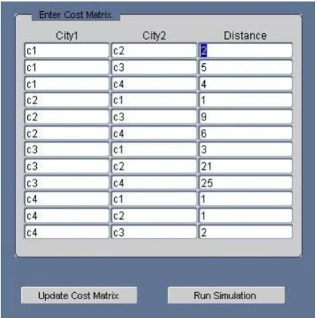
Fig 6 Cost matrix

Figure 6 shows the cost matrix of TSP for 4 cities. In this figure first column and second column represent the city denoted by C1, C2, C3 and C4. In third column we have distance between two cities, for example, first row represent the distance between city C1 and C2 is 2.

Fig 7 shortest distance with path

Figure 7 represents the result of dynamic programming approach. This shows the shortest distance and suggested path for traveling salesman.

5.

CONCLUSION

This paper discusses the survey of various available methods for solving the symmetric or asymmetric TSP. An algorithm and implementation of TSP using dynamic programming is presented. The advantageous of this approach is that it gives correct and optimal solution with complexity Ο(n22n). In

future we use heuristic as a intermediate step to find the optimal solution using dynamic programming approach.

6.

REFERENCES

[1] Applegate, D. L., Bixby, R. E., Chvảtal, V. & Cook, W. J. (2006). The Traveling Salesman Problem:

AComputational Study, Princeton University Press, Princeton, New Jersey.

[2] CormenT. H., Leiserson, C. E., Rivest, R. L. & Stein, C. (2001). Introduction to Algorithms, Second Edition, MIT Press Cambridge, Massachusetts.

[3] The Traveling Salesman Problem: A case study in local optimization by David S. Johnson and Lyle A. McGeoch 1995

[4] D.L. Applegate, R.E. Bixby, V.Chv´atal, W.J. Cook, The Traveling Salesman Problem, A Computational Study, Princeton University Press, Princeton and Oxford, 2006.

[5] http://en.wikipedia.org/wiki/Traveling_salesman_probl-em.

[6] Applegate, D. L., R. E. Bixby, V. Chvátal, and W. J. Cook (2007). The Traveling Salesman Problem: A Computational Study (Princeton Series in Applied Mathematics)., Chapter 1–5,12–17. Princeton, NJ, USA: Princeton University Press.

[7] Cook, William. "History of the TSP." The Traveling Salesman Problem. Oct 2009. Georgia Tech, 22 Jan 2010. <http://www.tsp.gatech.edu/index.html>.

[8] A Multilevel Scheme for the Traveling Salesman Problem Øystein M. Hjertenes University of Bergen 2002.

[9] V. Chachra, P.M. Ghare, J.M. Moore, Applications of Graph Theory Algorithms, Elsevier North Holland, Inc., 1979.

[10]Dantzig, G., R. Fulkerson, and S. Johnson (1954). Solution of a large scale traveling salesman problem. Technical Report P-510, RAND Corporation, Santa Monica, California, USA.

[11]Cook, William. "History of the TSP." The Traveling Salesman Problem. Oct 2009. Georgia Tech, 22 Jan 2010. <http://www.tsp.gatech.edu/index.html>.

[12]Karp, R. M. (1972). Reducibility among combinatorial problems. In R. Miller and J. Thatcher (Eds.), Complexity of Computer Computations, New York, USA., pp. 85–103. Plenum Press.

[13]Christofides, N. (1976). Worst-case analysis of a new heuristic for the traveling salesman problem. Technical Report Report 388, Graduate School of Industrial Administration, Carnegie-Mellon University, Pittsburg.

[14]S. Kirkpatrick, C. D. G. J. and M. P. Vecchi (1983, May). Optimization by simulated annealing. Science 220(4598), 671–680.

[15]Hopfield, J. J. and D. W. Tank (1985). “Neural” computation of decisions in optimization problems. Biological Cybernetics 52, 141–152. 10.1007/BF00339943.

Volume 52– No.4, August 2012

[17] http://www.iwr.uniheidelberg.de/groups/comopt/softwar-e/TSPLIB95/

[18]Reinelt, G. (1991, Fall). Tsplib - a traveling salesman problem library. ORSA, Journal On Computing 3(4), 376–384.

[19]G. Dantzig, R. Fulkerson, and S. Johnson. Solution of a large scale traveling salesman problem. Operations Research, 2:393–410, 1954.

[20]A. H. Land and A. Doig. An automatic method for solving discrete programming problems. Econometrica, 28:497–520, 1960.

[21]J. D. Little, K. G. Murty, D. W. Sweeney, and C. Karel. An algorithm for the traveling salesman problem. Operations Research, 11(6):972– 989, 1963.

[22]Okano, H. (2009). Study of Practical Solutions for Combinatorial Optimization Problems. Ph. D. thesis, School of Information Sciences, Tohoku University.

[23]Dantzig, G., Fulkerson, R., Johnson, S.: Solution of a large-scale traveling salesman problem. Operations Research 2, 393{410, 1954.

[24]http://en.wikipedia.org/wiki/Christofides_algorithm

[25]The Traveling Salesman Problem: A case study in local optimization by David S. Johnson and Lyle A. McGeoch 1995

[26]D. S. Johnson and L. A. McGeoch. The Traveling Salesman Problem: A Case Study. In E. H. Aarts and J. K. Lenstra, editors, Local Search in Combinatorial Optimization. Wiley and Sons, New York, NY, USA, 1997.

[27]The Traveling Salesman Problem: A case study in local optimization by David S. Johnson and Lyle A. MuGeoch 1995

[28]D. J. Rosenkrantz, R. E. Stearns, and P. M. Lewis, II, An analysis of several heuristics for the traveling salesman problem, SIAM J. Comput. 6 (1977), 563-581.

[29]G. Reinelt. The traveling salesman: Computational solutions for TSP applications. Springer Verlag, Berlin, Germany, 1994. LNCS 840.

[30]G. Reinelt. The traveling salesman: Computational solutions for TSP applications. Springer Verlag, Berlin, Germany, 1994. LNCS 840.

[31]A. M. Frieze, Worst-case analysis of algorithms for traveling salesman problems, Methods of Operations Research 32 (1979), 97-112.

[32]D.S. Johnson and L.A. McGeoch, “The TravelingSalesman Problem: A Case Study in Local Optimization”,November 20, 1995.

[33]G. Gutin and A. Yeo. Polynomial approximation algorithms for the TSP and the QAP with a factorial domination number. Discrete Applied Mathematics, 119(1-2):107–116, 2002.

[34]http://en.wikipedia.org/wiki/Hill_climbing

[35]S. Lin and B. Kernighan. An effective heuristic algorithm for the traveling-salesman problem. Operations Research, 21:498–516, 1973.

[36]S. Kirkpatrick, C. D. Gelatt Jr., and M. P. Vecchi. Optimization by simulated annealing. Science, 220(4598):671–680, 1983.

[37]I. A. Wood and T. Downs. Fast optimization by demon algorithms. In T. Downs, M. Frean, and M. Gallagher, editors, Proceedings of the Ninth Australian Conference on Neural Networks (ACNN98), Queensland, Australia, pages 245–249, 1989.

[38]S. Kirkpatrick, C. Gelatt, and M. Vecchi. Optimization by simulated annealing. Science, 220(4598):671–680, 1983.

[39]N. Metropolis, A. Rosenbluth, M. Rosenbluth, A. Teller, and E. Teller. Equation of state calculations by fast computing machines. Journal of Chemical Physics, 21(6):1087–1092, 1953.

[40]R. W. Eglese. Simulated annealing: A tool for operational research. European Journal of Operational Research, 46(3):271–281, 1990.

[41]F. Glover. Heuristics for integer programming using surrogate constraints. Decision Sciences, 8(1):156–166, 1977.

[42]M. Dorigo, V. Maniezzo, and A. Colorni. The ant system: Ant autocatalytic optimizing process. Technical Report TR91-016, Politenico di Milano, 1991.

[43]M. Dorigo, G. Di Caro, and L. M. Gambardella. Ant algorithms for discrete optimization.Artificial Life, 5(2):137–172, 1999

[44]A. Fraser. Simulation of genetic systems by automatic digital computers. I. introduction. Australian Journal of Biological Science, 10:484–491, 1957.

[45]A. Fraser. Simulation of genetic systems by automatic digital computers. II. Effects of linkage on rates of advanced under-selection. Australian Journal of Biological Science, 10:492–499, 1957.