A Methodology for Neural Spatial Interaction Modeling

Munich Personal RePEc Archive

A Methodology for Neural Spatial

Interaction Modeling

Fischer, Manfred M. and Reismann, Martin

Vienna University of Economics and Business, Vienna University of

Economics and Business

2002

Online at

https://mpra.ub.uni-muenchen.de/77794/

Manfred M. Fischer and Martin Reismann

A Methodology for

Neural Spatial Interaction Modeling

This paper attempts to develop a mathematically rigid and unified framework for

neural spatial interaction modeling. Families of classical neural network models, but

also less classical ones such as product unit neural network ones are considered for the

cases of unconstrained and singly constrained spatial interaction flows. Current

practice appears to suffer from least squares and normality assumptions that ignore the

true integer nature of the flows and approximate a discrete-valued process by an

almost certainly misrepresentative continuous distribution. To overcome this deficiency

we suggest a more suitable estimation approach, maximum likelihood estimation under

more realistic distributional assumptions of Poisson processes, and utilize a global

search procedure, called Alopex, to solve the maximum likelihood estimation problem.

To identify the transition from underfitting to overfitting we split the data into training,

internal validation and test sets. The bootstrapping pairs approach with replacement is

adopted to combine the purity of data splitting with the power of a resampling

procedure to overcome the generally neglected issue of fixed data splitting and the

problem of scarce data. In addition, the approach has power to provide a better

statistical picture of the prediction variability, Finally, a benchmark comparison

against the classical gravity models illustrates the superiority of both, the

unconstrained and the origin constrained neural network model versions in terms of

generalization performance measured by Kullback and Leibler’s information criterion.

The authors gratefully acknowledge the grant no. P15575 provided by the Austrian Fonds zur Förderung

der wissenschaftlichen Forschung (FWF).

Manfred M. Fischer is Chaired Professor of the Department of Economic Geography &

E-Martin Reismann is research assistant at the same department. E-mail:

There are several phases that an emerging field goes through before it reaches

maturity, and GeoComputation is no exception. There is usually a trigger for birth of

the field. In our case, new techniques such as neural networks and evolutionary

computation, significant progress in computing technology, and the emerging data rich

environment inspired many scholars to revisit old and tackle new spatial problems. The

result has been a wealth of new approaches, with significant improvements in many

cases (see Longley et al. 1998, Fischer and Leung 2001).

After the initial excitement settles in, the crest breaking question is whether the new

community of researchers can produce sufficient results to sustain the field, and

whether practitioners will find these results to be of quality, novelty, and relevance to

make a real impact. Successful applications of geocomputational models and

techniques to a variety of problems such as data mining, pattern recognition,

optimization, traffic forecasting and spatial interaction modeling rang the bell

signifying the entry of GeoComputation as an established field.

This paper is a response to the perceived omission in the comprehensive

understanding of one of the most important subfields in GeoComputation. While

various papers on neural network modeling of unconstrained spatial interaction flows

have appeared in the past decade, there has yet to be an advanced discussion of the

general concepts involved in the application of such models. This paper attempts to fill

the gap. Among the elements which should be of interest to those interested in

applications are estimation and performance issues.

The paper proceeds as follows. The first section points to some shortcomings evident in

current practice and motivates to depart in two directions: First, to employ maximum

likelihood under more realistic distributional assumptions rather than least squares and

normality assumptions, and second to utilize bootstrapping to overcome the problems

of fixed data splitting and the scarcity of data that affect performance and reliability of

the model results. Section 2 describes classical unconstrained neural spatial interaction

models and less classical ones. Classical models are those that are constructed using a

single hidden layer of summation units. In these network models each input to the

product unit rather than the standard summation neural network framework for

modeling interactions over space.

Unconstrained – summation unit and product unit – neural spatial interaction

models represent rich and flexible families of spatial interaction function

approximators. But they may be of little practical value if a priori information is

available on accounting constraints on the predicted flows. Section 3 moves to the case

of constrained spatial interaction. To satisfactorily tackle this issue within a neural

network environment it is necessary to embed the constraint-handling mechanism

within the model structure. This is a far from easy task. We briefly describe the only

existing generic model approach for the single constrained case (see Fischer, Reismann

and Hlavackova-Schindler 2001), and present summation and product unit model

versions. We reserve the doubly constrained case to subsequent work.

We view parameter estimation (network learning) in an optimization context and

develop a rationale for an appropriate objective (loss) function for the estimation

approach in Section 4. Global search procedures such as simulated annealing or Alopex

may be employed to solve the maximum likelihood estimation problem. We follow

Fischer, Hlavackova-Schindler and Reismann (2001) to utilize the Alopex procedure

that differs from the method of simulated annealing in three important aspects. First,

correlations between changes in individual parameters and changes in the loss function

are used rather than changes in the loss function only. Second, all parameter changes

are accepted at every iteration, and, third, during an iteration step all parameters are

updated simultaneously.

The standard approach to evaluate the generalization performance of neural network

models is to split the data set into three subsets: the training set, the internal validation

set and the testing set. It has become common practice to fix these sets. A bootstrapping

approach is suggested to overcome the generally neglected problem of sensitivity to the

specific splitting of the data, and to get a better statistical picture of prediction

variability of the models. Section 5 illustrates the application of the various families of

neural spatial interaction function approximators discussed in the previous sections, and

presents the results of a comparison of the performance of the summation and the

cases] against the corresponding standard gravity models. The testbed for the evaluation

uses interregional telecommunication traffic data from Austria. Section 6 outlines some

directions for future research.

1. DEPARTURES FROM CURRENT PRACTICE

We will begin our analysis with the simplest case, namely that of unconstrained spatial

interaction. For concreteness and simplicity, we consider neural spatial interaction

models based on the theory of single hidden layer feedforward models. Current

research in this field appears to suffer from least squares and Gaussian assumptions that

ignore the true integer nature of the flows and approximate a discrete-valued process by

an almost certainly misrepresentative distribution. As a result, least squares estimates

and their standard errors can be seriously distorted. To overcome this shortcoming we

will develop a more appropriate estimation approach under more realistic distributional

assumptions.

Thus, throughout the paper we assume observations generated as the realization of a

sequence

{

Zk =

(

X Yk, k

)

,k =1,...,K

}

of

(

N+ ×1

)

1 vectors

(

N∈

)

defined on a

Poisson probability space. The random variables Y_k represent targets. Their relationship

to the variables X_k is of primary interest. When E Y

( )

_k < ∞, the conditional

expectation of Y_k given X_k exists, denoted as g =E Y X

(

_{k k}

)

. Defining

( )

k Yk Xk

ε ≡ −g , we can also write Y_k =g

( )

X_k +ε_k. The unknown spatial interaction

function g embodies the systematic part of the stochastic relation between Y_k and X_k.

The error ε_k is noise, with the property that E

(

ε_k X_k

)

=0 by construction. Our

problem is to learn (estimate, approximate) the mapping g from a realization of the

sequence

{ }

Z_k .

In practice, we observe a realization of only a finite part of the sequence

{ }

Z_k , a

training set or sample of size K (i.e. a realization of

{

Z k_k =1,...,K

}

). Because g is an

element of a space of spatial interaction functions, say G , we have essentially no hope

of learning g in any complete sense from a sample of fixed finite size. Nevertheless, it

is possible to approximate g to some degree of accuracy using a sample of size K, and

There are many standard procedures of function approximation to this function g.

Perhaps the simplest is linear regression. Since feedforward neural networks are

characteristically nonlinear it is useful to view them as performing a kind of nonlinear

regression. Several of the issues that come up in regression analysis are also relevant to

the kind of nonlinear regression performed by neural networks.

One important example comes up in the cases of underfitting and overfitting. If the

neural network model is able to approximate only a narrow range of functions, then it

may be incapable of approximating the true spatial interaction function no matter how

much training data is available. Thus, the model will be biased, and it is said to be

underfitted. The solution to this problem seems to be to increase the complexity of the

neural network, and, thus, the range of spatial interaction functions, that can be

approximated, until the bias becomes negligible. But, if the complexity [too many

degrees of freedom] rises too far, then overfitting may arise and the fitted model will

again lead to poor estimates of the spatial interaction function. If overfitting occurs then

the fitted model can change significantly as single training samples are perturbed and,

thus shows high variance. The ultimate measure of success is not how closely the

model approximates the training data, but how well it accounts for not yet seen cases.

Optimizing the generalization performance requires that the neural network complexity

is adjusted to minimize both the bias and the variance as much as possible.

Since the training data will be fitted more closely as the model complexity increases,

the ability of the trained model to predict this data cannot be utilized to identify the

transition from underfitting to overfitting. In order to choose a suitably complex model,

some means of directly estimating the generalization performance are needed. For

neural spatial interaction models data splitting is commonly used. Though this

procedure is simple to use in practice, effective use of data splitting may require a

significant reduction in the amount of data which is available to train the model. If the

available data is limited and sparsely distributed – and this tends to be the rule rather

than the exception in spatial interaction contexts, then any reduction in amount of

training data may obscure or remove features of the true spatial interaction function

In this contribution, we address this issue by adopting the bootstrapping pairs approach

(see Efron 1982) with replacement. This approach will combine the purity of data

splitting with the power of a resampling procedure and, moreover, allows to get a better

statistical picture of the prediction variability. An additional benefit of the bootstrap is

that it provides approximations to the sampling distribution of the test statistic of

interest that are considerably more accurate than the analytically obtained large sample

approximations. Formal investigation of this additional benefit is beyond the scope of

this contribution. We have a full agenda just to analyze the performance of summation

and product unit neural network models for the cases of unconstrained and constrained

spatial interaction. But we anticipate that our bootstrapping procedure may well afford

such superior finite sample approximations.

2. FAMILIES OF UNCONSTRAINED NEURAL SPATIAL INTERACTION

MODELS

In many spatial interaction contexts, little is known about the form of the spatial

interaction function which is to be approximated. In such cases it is generally not

possible to use a parametric modeling approach where a mathematical model is

specified with unknown coefficients which have to be estimated to fit the model. The

ability of neural spatial interaction models to model a wide range of spatial interaction

functions relieves the model user of the need to specify exactly a model that includes all

the necessary terms to model the true spatial interaction function.

The Case of Unconstrained Spatial Interaction

There is a growing literature in geography and regional science that deals with

alternative model specifications and estimators for solving unconstrained spatial

interaction problems. Examples include, among others, Fischer and Gopal (1994);

Black (1995); Nijkamp, Reggiani and Tritapepe (1996); Bergkvist and Westin (1997);

Bergkvist (2000); Reggiani and Tritapepe (2000); Thill and Mozolin (2000); Mozolin,

Thill and Usery (2000). All these models are members of the following general class of

(

)

00 0 1

1 1

,

H N

H H

h hn n

h n

w w w x

Ω ψ ϕ

= =

  

= _ + _{ }

 



∑

∑



x w (1)

where the N-dimensional euclidean space (generally, N = 3) is the input space and the

1-dimensional euclidean space the output space. Vector x=

(

x₁,...,x_N

)

is the input vector that represents measures characterizing the origin and the destination of spatial

interaction as well as their separation. H ≡

(

₀, ₁

)

w w w is the

(

HN+ + ×H 1

)

1 vector of

the network weights (parameters). There are H hidden units. The vector w₀ contains

the hidden to output unit weights, w₀ ≡

(

w₀₀,w₀₁,...,w_0H

)

, and the vector w₁ contains the input to hidden unit weights, w₁≡

(

w₁₀,...,w_1H

)

with w_1h ≡

(

w_{1 1h} ,...,w_1hN

)

. We allow a bias at the hidden layer by including w₀₀. A bias at the input array may be taken into

consideration by setting x₁≡1. ϕ is a hidden layer transfer function, ψ an output unit transfer function, both continuously differentiable of order 2 on ℜ. Note that the model

output function and the weight vector are explicitly indexed by the number, H, of

hidden units in order to indicate the dependence. But to simplify notation we drop the

superindex hereafter.

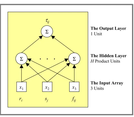
FIGURE 1 TO BE PLACED ABOUT HERE

FIG. 1 depicts the corresponding network architecture. Hidden units, denoted by the

symbol Σ, indicate that each input is multiplied by a weight and then summed. Thus,

models of type (1) may be termed unconstrained summation unit spatial interaction

models. The family of approximations (1) embodies several concepts already familiar

from the pattern recognition literature. It is the combination of these that is novel.

Specifically, ₁

1

N

hn n n= w x

∑

is a familiar linear discriminant function (see Young and

Calvert 1974) which – when transformed by ϕ – acts as a nonlinear feature detector.

The 'hidden' features are then subjected to a linear discriminant function and filtered

through ψ . The approximation benefits from the use of nonlinear feature detectors,

while retaining many of the advantages of linearity in a particularly elegant manner.

A leading case occurs when both transfer functions are specified as logistic

(

)

1 1

00 0 1

1 1

, 1 exp 1 exp

H N

L h hn n

h n

w w w x

Ω − − = =    _{  }   _{  } = +_ − + _ + _− _{ }         _{  } 

∑

∑



x w (2)

that has been often used in practice (see, for example, Mozolin, Thill and Usery 2000;

Fischer, Hlavackova-Schindler and Reismann 1999; Fischer and Leung 1998; Gopal

and Fischer 1996; Black 1995; Fischer and Gopal 1994; Gopal and Fischer 1993;

Openshaw 1993).

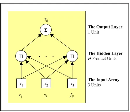
Product Unit Model Versions

Neural spatial interaction models of type (1) are constructed using a single hidden layer

of summation units. In these networks each input to the hidden node is multiplied by a

weight and then summed. A nonlinear transfer function, such as the logistic function, is

employed at the hidden layer. Neural network approximation theory has shown the

attractivity of such summation networks.

In the neural network community it is well known that supplementing the inputs to a

neural network model with higher-order combinations of the inputs increases the

capacity of the network in an information capacity sense (see Cover 1965) and its

ability to learn (see Giles and Maxwell 1987). This may motivate to utilize a product

unit rather than the standard summation unit neural network framework for modeling

interactions over space. The general class of unconstrained product unit spatial

interaction models is given as

(

)

1

00 0 1 1 , hn N H w h n h n

w w x

π_{Ω ψ ϕ}

= =

  

= _ + _{ }

 



∑

∏



x w (3)

which contain both product and summation units. The product units compute the

product of inputs, each raised to a variable power. FIG. 2 illustrates the corresponding

network architecture.

Specifying ϕ

( )

⋅ to be the identity function and ψ

( )

⋅ to be the logistic function we

obtain the following special case of (3)

(

)

1

1

00 0

1 1

, 1 exp hn

N H

w

L h n

h n

w w x

π_Ω

−

= =

    

 

= + − +  

 

 

  



∑

∏



x w (4)

3. NEURAL NETWORKS OF CONSTRAINED SPATIAL INTERACTION

FLOWS

Classical neural network models of the form (1) and less classical models of the type

(3) represent rich and flexible families of neural spatial interaction approximators. But

they may be of little practical value if a priori information is available on accounting

constraints of the predicted flows. For this purpose Fischer, Reismann and

Hlavackova-Schindler (2001) have recently developed a novel class of neural spatial interaction

models that are able to deal efficiently with the singly constrained case of spatial

interaction.

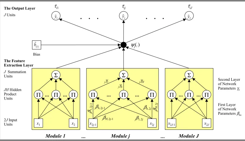
The models are based on a modular connectionist architecture that may be viewed

as a linked collection of functionally independent modules with identical feedforward

topologies [two inputs, H hidden product units and a single summation unit], operating

under supervised learning algorithms. The prediction is achieved by combining the

outcome of the individual modules using a nonlinear output transfer function multiplied

with a bias term that implements the accounting constraint.

Without loss of generality we consider the origin constrained model version only. FIG.

3 illustrates the modular network architecture of the models. Modularity is seen here as

decomposition on the computational level. The network is composed of two processing

layers and two layers of network parameters. The first processing layer is involved with

the extraction of features from the input data. This layer is implemented as a layer of J

functionally independent modules with identical topologies. Each module is a

feedforward network with two inputs x_2j−1 and x_2j[representing measures of

H hidden product units, denoted by the symbol Π, and terminates with a single

summation unit, denoted by the symbol Σ. The collective output of these modules

constitutes the input to the second processing layer consisting of J output units that

[image:12.595.121.356.645.712.2]

perform the flow prediction.

FIGURE 3 TO BE PLACED ABOUT HERE

This network architecture implements the general class of product unit neural

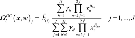
models of origin constrained [OC] spatial interaction

(

)

2

1 2 1

, hn 1, ...,

j H

OC

j h h n

j

h n j

xβ j J

π_{Ω ψ γ ϕ}

= = −

  

= _  _ =

 



∑

∏



x w (5)

with :ϕ_h ℜ → ℜ,ψ_j:ℜ → ℜ and x∈ℜ2J, that is x=

(

x x₁, ₂, ...,x_2j−1,x_2j, ...,x_2J−1,x_2J

)

where x_2j−1 represents a variable pertaining to destination j

(

j=1, ...,J

)

and x_2j a variable f_ij pertaining to the separation from region i to region j

(

i=1, ..., ;I j=1, ...,J

)

of the spatial interaction system under scrutiny. β_hn

(

h=1, ...,H n; =2j−1, 2j

)

are the input-to-hidden connection weights, and γ_h

(

h=1, ...,H

)

the hidden-to-output weights

in the j-th module of the network model. The symbol w is a convenient shorthand

notation of the (3H)-dimensional vector of all the model parameters. ψ_j

(

j=1, ...,J

)

represents a nonlinear summation unit transfer function and ϕ_h

(

h=1,...,H

)

a linear hidden product unit transfer function.

Specifying ϕ_h

( )

⋅ to be the identity function and ϕ_j

( )

⋅ a nonlinear normalized

function we obtain the following important special case of (5)

(

)

( )

2

1 2 1 2

1 1 2 1

, 1, ...,

hn

h n

j H

h n

h n j OC

1 j i J H j

h n

j h n j x

b j J

where b_{( )i} is the bias signal that can be thought as being generated by a ’dummy unit’

whose output is clamped at the scalar t_ii A more detailed description of the model may

be found in Fischer, Hlavackova-Schindler and Reismann (2001).

Summation Unit Model Versions

The summation unit version of the general class of product unit neural network

models of origin constrained spatial interaction may be easily derived from Equation

(5):

(

)

2

1 2 1

, 1, ...,

j H

OC

j h h hn n

j

h n j

x j J

Σ_{Ω ψ γ ϕ β}

= = −

  

= _  _ =

 



∑

∑



x w (7)

where :ϕh ℜ → ℜ, :ψj ℜ → ℜ and

2J

∈ℜ

x as above. Specifying ϕh

( )

⋅ as logistic

function for h = 1,...,N, and ψ_j

( )

⋅ as nonlinear normalized output transfer function we

obtain the following origin constrained member of class (7)

(

)

( )

1 2

1 2 1

1 2

1 1 2 1

1 exp

, 1, ...,

1 exp

j H

h hn n

h n j

OC

1 j i

j J H

h h n n

j h n j

x

b j J

x Σ γ β Ω γ β − = = − − = = = −    + −     _{ }   = =    + −     _{ }  

∑

∑

∑∑

∑

x w ' ' ' ' ' ' (8)

4. A RATIONALE FOR THE ESTIMATION APPROACH

If we view a neural spatial interaction model, unconstrained or constrained, as

generating a family of approximations (as w ranges over W, say) to a spatial

interaction function g , then we need a way to pick a best approximation from this

family. This is the function of network learning (training, parameter estimation) which

might be viewed as an optimization problem.

We develop a rationale for an appropriate objective (loss, cost) function for this task.

is the most likely explanation of the observed data set, say M. We can express this as

attempting to maximize the term

( )

(

)

P M

(

( )

_{( )}

)

P

(

( )

)

P M

P M

Ω

Ω w = w Ω w (9)

where Ω represents the neural spatial interaction model (with all the weights wH) in question, unconstrained or constrained. P M

(

Ω

( )

w

)

is the probability that the model

would have produced the observed data M . Since sums are easier to work with than

products, we will maximize the log of this probability, and since this log is a monotonic

transformation, maximizing the log is equivalent to maximizing the probability itself. In

this case we have

( )

(

)

(

( )

)

(

( )

)

( )

lnP Ω w M =lnP M Ω w +lnP Ω w −lnP M (10)

The probability of the data,P M

( )

, is not dependent on the model. Thus, it is

sufficient to maximize lnP M

(

Ω

( )

w

)

+lnP

(

Ω

( )

w

)

. The first of these terms

represents the probability of the data given the model, and hence measures how well the

network accounts for the data. The second term is a representation of the model itself;

that is, it is a prior probability, that can be utilized to get information and constraints

into the learning procedure.

We focus solely on the first term, the performance, and begin by noting that the data

can be broken down into a set of observations, M =

{

z_k =

(

x y_k, _k

)

k=1,...,K

}

, each z_k,

we will assume, chosen independently of the others. Hence we can write the probability

of the data given the model as

( )

(

)

(

( )

)

(

( )

)

ln ln _k ln _k

k k

P M Ω w =

∏

P z Ω w =

∑

P z Ω w (11)

Note that this assumption permits to express the probability of the data given the model

given the model. We can still take another step and break the data into two parts: the

observed input data x_k and the observed target y_k. Therefore we can write

( )

(

)

(

( )

)

( )

ln ln _{k k} and _k ln _k

k k

P M Ω w =

∑

P y x P xΩ w +

∑

(12)

Since we assume that x_k does not depend on the model, the second term of the equation

will not affect the determination of the optimal model. Thus, we need only to maximize

the term ln

(

_{k k} and

( )

)

k P y x Ω

∑

w .

Up to now we have – in effect – made only the assumption of the independence of

the observed data. In order to proceed, we need to make some more specific

assumptions, especially about the relationship between the observed input data x_k and

the observed target data y_k, a probabilistic assumption. We assume that the relationship

between x_k and y_k is not deterministic, but that for any given x_k there is a distribution

of possible values of y_k. But the model is deterministic, so rather than attempting to

predict the actual outcome we only attempt to predict the expected valued of y_k given

k

x . Therefore, the model output is to be interpreted as the mean bilateral interaction

frequencies (that is, those from the region of origin to the region of destination). This is,

of course, the standard assumption.

To proceed further, we have to specify the form of the distribution of which the

model output is the mean. Of particular interest to us is the assumption that the

observed data are the realization of a sequence of independent Poisson random

variables. Under this assumption we can write the probability of the data given the

model as

( )

(

and

)

( )

exp

(

( )

)

!

k

y

k k

k

k k _k

k P y x

y

Ω Ω

Ω =

∏

−

w w

w (13)

and, hence, define a maximum likelihood estimator as a parameter vector ˆw which

(

)

(

( )

( )

)

max L , , max _k yklnΩ _k Ω _k

∈ = ∈

∑

−

w W x y w w W w w (14)

Instead of maximizing the log-likelihood it is more convenient to view learning as

solving the minimization problem

(

)

(

)

min , , min L , ,

∈ = ∈ − 

w W w W

x y w x y w

λ (15)

where the loss (cost) function λ is the negative log-likelihood L. λ is non-negative,

continuously differentiable on the Q-dimensional parameter space (Q=HN+ +H 1 in

the unconstrained case and Q=3Hin the constrained one) which is a finite dimensional

closed bounded domain and, thus, compact. It can be shown that λ assumes its value as

the weight minimum under certain conditions.

5. TRAINING THE NEURAL NETWORK MODELS

Since the loss function λ is a complex nonlinear function of w for the neural

spatial interaction models, ˆw cannot be found analytically and computationally

intensive iterative optimization techniques such as global search procedures must be

utilized to find (15). Simulated annealing, genetic algorithms and the Alopex2

procedure are attractive candidates for this task. We utilize the latter as described in

Fischer, Hlavackova-Schindler and Reismann (2001).

The loss function λ

( )

w is minimized by means of weight changes that are

computed for the s-th step (s>2) of the iteration process as follows3,

( )

(

1

)

( )

k k k

w s =w s− +δ s (16)

where δ_k

( )

s is a small positive or negative step of size δ with the following

( )

_{with probability 1}with probability k

( )

_{( )}

k k p s s p s δ

δ =₊−_{δ  − }

  

 (17)

The probability pk

( )

s for a negative step is given by the Boltzmann distribution

( )

(

( ) ( )

)

1

1 exp /

k k

p s = +_ −C s T s _− (18)

where

( )

( )

( )

k k

C s = ∆w s ∆λ s (19)

with

( )

(

1

)

(

2

)

k k k

w s w s w s

∆ = − − − (20)

and

( )

s

(

s 1

) (

s 2

)

λ λ λ

∆ = − − − (21)

The parameter T in Equation (18), termed temperature in analogy to simulated

annealing, is updated using the following annealing schedule:

( )

( )

(

)

1

if is a multiple of

1 otherwise

s

k k s s S

C s s S

QS T s T s δ − = −   =  ₋ 

∑ ∑

' ' (22)

where (Q=HN+ +H 1 in the case of the unconstrained models, and Q=3H in the

case of the constrained models) denotes the number of weights. When T is small, the

probability of changing the parameters is around zero if Ck is negative and around one

The effectiveness of Alopex in locating global minima and its speed of convergence

critically depend on the balance of the size of the feedback term ∆ ∆w_k λ and the

temperature T. If T is very large compared to ∆ ∆w_k λ the process does not converge. If

T is too small, a premature convergence to a local minimum might occur. The

procedure is governed by three parameters: the initial temperature T, the number of

iterations, S, over which the correlations are averaged for annealing, and the step size

δ. The temperature T and the S-iterations cycles seem to be of secondary importance

for the final performance of the algorithm. The initial temperature T may be set to a

large value of about 1,000. This allows the algorithm to get an estimate of the average

correlation in the first S iterations and reset it to an appropriate value according to

Equation (22). S may be chosen between 10 and 100. In contrast to T and S, δ is a

critical parameter that has to be selected heuristically with care. There is no way to a

priori identify δ in the case of multimodal parameter spaces.

The Termination Criterion

It has been observed that forceful training may not produce network models with

adequate generalization ability, although the learning error achieved is small. The most

common remedy for this problem is to monitor model performance during training to

assure that further training improves generalization as well. For this purpose an

additional set of validation data, independent from the training data is used. In a typical

training phase, it is normal for the validation error to decrease. This trend may not be

permanent, however. At some point the validation error usually reverses. Then the

training process should be stopped. In our implementation of the Alopex procedure

network training is stopped when κ =40, 000 consecutive iterations are unsuccessful.

κ has been chosen so large at the expense of the greater training time, to ensure more reliable estimates.

6. EXPERIMENTAL ENVIRONMENT, PERFORMANCE TESTS AND

BENCHMARK COMPARISONS

To illustrate the application of modeling and estimation tools discussed in the

The Benchmark Models

The standard unconstrained gravity model

1,..., ; 1,..., ;

grav

ij k ri s dj ij i I j J j i

α β γ

τ ₌ − _{= = ≠ (23)}

with

i j ij i j j

t k

r s dα β −γ

≠ =

∑∑

ii (24)

: _ij

i j j

t t

≠

=

∑∑

ii (25)

serves as a benchmark model for the unconstrained neural spatial interaction models4,

that is, the classical models of type (2) and the less classical ones of type (4). grav ij

τ denotes the estimated flow from i to j, k is a factor independent of all origins and

destinations, α reflects the relationship of r_i with grav ij

τ and β the relationship of s_j

with τ_ijgrav. γ is the distance sensitivity parameter, γ >0. r_i and s_j are measured in

terms of the gross regional product, d_ij in terms of distances from i to j, whereas t_ij in

terms of erlang (see Fischer and Gopal 1994 for more details).

The standard origin constrained gravity model

( ) 1,... ; 1,..., ;

orig grav

ij bi sj dij i I j J j i

α γ

τ ₌ − _{= = ≠ (26)}

with

( )i i j ij j i

t b

s dα −γ

≠

=

∑

i (27)

: i ij j i t t ≠ =

∑

i (28)

is used as benchmark model for the constrained neural spatial interaction models (6)

and (8). b_{( )i} is the origin specific balancing factor. , ,α γ s_j, d_ij and t_ij are defined as

above.

Performance Measure

One needs to be very careful when selecting a measure to compare different models.

It makes not much sense to utilize least squares related performance measures, such as

the average relative variances or the standardized root mean square, in the context of

our ML estimation approach. Model performance is measured in this study by means of

Kullback and Leibler’s (1951) information criterion (KLIC) which is a natural

performance criterion for the goodness-of-fit of ML estimated models:

( )

(

)

(

)

1 ' ' 1 1 1 ' _'

' 1 _{' 1}

ln , , Ω Ω − = − = = ₌  _{ }   _{ }      = _{ }    _{ }       

∑

∑

∑

_∑

U u u U u u U _U u

u _{u u}

u _u

y y

y KLIC M

y _{x w x w}

(29)

where

(

x yu, u

)

denotes the u-th pattern of the data set M , and Ω is the neural spatial

interaction model under consideration. The performance measure has a minimum at

zero and a maximum at positive infinity when yu >0 and Ω

( )

xuw =0 for any

(

x yu, u

)

pair.

The Data, Data Splitting and Bootstrapping

To model interregional telecommunication flows for Austria we utilize three

Austrian data sources – a (32, 32)-interregional telecommunication flow matrix

( )

tij , a

(32, 32)-distance matrix

( )

d_ij , and gross regional products for the 32

telecommunication regions – to produce a set of 992 4-tupel

(

r s d ti, j, ij; ij

)

with

(

)

, 1,...,32

2j 1

x ₋ and x_2j of the j-th module of the origin constrained network models, and the last

component the target output. The bias term b_{( )i} is clamped to the scalar t_ii. s_j

represents the potential draw of telecommunication in j and is measured in terms of the

gross regional product, d_ij denotes distances from i to j, while t_ij represents

telecommunication traffic flows. The input data5 were rescaled to lie in [0.1, 0.9].

The telecommunication data stem from network measurements of carried traffic in

Austria in 1991, in terms of erlang, an internationally widely used measure of

telecommunication contact intensity, which is defined as the number of phone calls

(including facsimile transfers) multiplied by the average length of the call (transfer)

divided by the duration of measurement(for more details, see Fischer and Gopal 1994).

The data refer to the telecommunication traffic between the 32 telecommunication

districts representing the second level of the hierarchical structure of the Austrian

telecommunication network. Due to measurement problems, intraregional traffic (i.e.

i = j) is left out of consideration.

The standard approach to evaluate the out-of-sample [prediction] performance of a

neural spatial interaction model (see Fischer and Gopal 1994) is to split the total data

set M of 992 samples into three subsets: the training [in-sample] set

(

)

{

}

1 u1, u1 with 1 1,..., 1 496 patterns

M = x y u = U = , the internal validation set

(

)

{

}

2 u2, u2 with 2 1,..., 2 248 patterns

M = x y u = U = and the testing [prediction,

out-of-sample] set M₃=

{

(

xu₃,yu₃

)

with 3 1,...,u = U₃ =248 patterns

}

. M1 is used only for

parameter estimation, while M₂ for validation. The generalization performance of the

model is assessed on the testing set M₃. It has become common practice to fix these

sets. But recent experience has found this approach to be very sensitive to the specific

splitting of the data. To overcome this problem as well as the problem of scarce data we

make use of the bootstrapping pairs approach (Efron 1982) with replacement. This

approach combines the purity of splitting the data into three disjoint data sets with the

power of a resampling procedure and allows us also to get a better statistical picture of

the prediction variability.

The idea behind this approach is to generate B pseudo-replicates of the training,

validation and test sets, then to re-estimate the model parameters w on each training

out-of-sample performance of the test bootstrap out-of-samples. In this bootstrap world, the errors of

prediction and the errors in the parameter estimates are directly observable. Statistics on

parameter reliability can easily be computed.

Implementing the approach involves the following steps (see Fischer and Reismann

2000):

Step 1: Conduct three totally independent re-sampling operations in which B

independent training bootstrap samples, B independent validation bootstrap

samples and B independent testing bootstrap samples are generated, by

randomly sampling U₁, U₂ and U₃ times, respectively, with replacement

from the observed input-output pairs M.

Step 2: For each training bootstrap sample the minimization problem (15) is solved

by applying the Alopex procedure. During the training process the KLIC

performance of the model is monitored on the corresponding bootstrap

validation set. The training process is stopped as specified in Section 5.

Step 3: Calculate the KLIC-statistic of generalization performance for each test

bootstrap sample. The distribution of the pseudo-errors can be computed,

and used to approximate the distribution of the real errors. This

approximation is the bootstrap.

Step 4: The variability of the B bootstrap KLIC-statistics gives an estimate of the

expected accuracy of the model performance. Thus, the standard errors of

the generalization performance statistic is given by the sample standard

deviation of the B bootstrap replications.

Performance Tests and Results

We consider first

to model the unconstrained case of spatial interaction, and then

• the modular product unit neural network version πΩ₁OC [see Equation (6)] and

• the modular summation unit neural network version OC

1

Σ_{Ω [see Equation (8)]}

of singly constrained neural spatial interaction models to model the origin constrained

case. Conventional gravity model specifications [see Equations (23)-(25) for the

unconstrained case and Equations (26)-(28) for the origin constrained case] serve as

benchmark models.

All the models were calibrated by means of the ML-estimation approach utilizing

the Alopex procedure to eliminate the effect of different estimation procedures on the

result. In order to do justice to each model specification, the critical Alopex parameter

δ [step size] was systematically sought for each model. The Alopex parameters T and

S were set to 1,000 and 10, respectively. We made use of the bootstrapping pairs

approach [B = 60] to overcome the problem of sensitivity to the specific splitting of the

data into in-sample, internal validation and generalization data sets, and the scarcity of

data, but also to get a better statistical picture of prediction variability.

It should be emphasized that the main goal of training is to minimize the loss

function λ. But it has been observed that forceful training may not produce network

models with adequate generalization ability. We adopted the most common remedy for

this problem and checked the model performance in terms of KLIC M

( )

₂ periodically

during training to assure that further training improves generalization, the so-called

cross-validation technique.

Alopex is an iterative procedure. In practice, this means that the final results of

training may vary as the initial weight settings are changed. Typically, the likelihood

functions of feedforward neural network models have many local minima. This implies

that the training process is sensitive to its starting point. Despite recent progress in

finding the most appropriate parameter initialization that would help Alopex – but also

other iterative procedures – to find near optimal solutions, the most widely adopted

approach still uses random weight initialization. In our experiments random numbers

The order of the input data presentation was kept constant for each run to eliminate its

effect on the result.

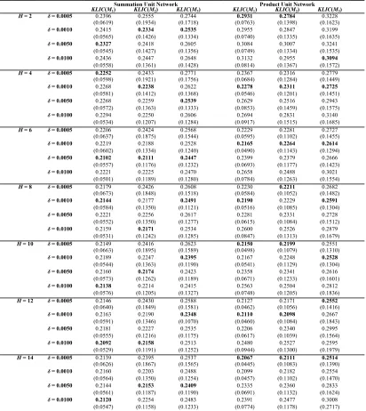
The Case of Unconstrained Spatial Interactions: Extensive computational experiments

with different combinations of H- and δ -values have been performed on DEC Alpha

375 Mhz, with H∈

{

2, 4, 6,8,10,12,14

}

and

{

0.0005, 0.0010, 0.0025, 0.0050, 0.0100, 0.0250, 0.0500, 0.1000

}

δ∈ . Selected results of

these experiments

[

H =2, 4, 6,8,10,12,14 and δ =0.0005, 0.0010, 0.0050, 0.0100

]

are

reported in TABLE 1. Training performance is measured in terms of KLIC M

( )

1 ,

validation performance in terms of KLIC M

( )

2 and testing performance in terms of

( )

3

KLIC M . The performance values represent the mean of B=60 bootstrap replications, standard deviations are given in brackets.

PLACE TABLE 1 ABOUT HERE

Some considerations are worth making. First, the best result (averaged over the 60

independent simulation runs) in terms of average out-of-sample KLIC-performance was

obtained with H =12 and δ =0.0010 in the case of the summation unit neural network model, and with H =14 and δ =0.0005 in the case of the product unit neural network

model. Second, there is convincing evidence that the summation unit model

outperforms the product unit model version at any given level of model complexity.

This is primarily due to the fact that the input data of Ω_L were preprocessed to

logarithmically transformed data scaled to [0.1, 0.9]. Third, it can be seen that model

approximation improves as the complexity of πΩ_L grows with increasing H (except H =

12). This appears to be less evident in the case of the summation unit model version.

Fourth, the experiments also suggest that δ =0.0010 tends to yield the best or at least rather good generalization performances in both cases of neural network models. The

poorest generalization performance of the summation unit network is obtained for

0.0005

δ = (except: H = 8) while δ =0.0100 leads to the poorest results in the case of

the product unit network model (except H = 2 and 12). Fifth, as already mentioned

above, forceful training may not produce the network model with the best

generalization ability. This is evidenced for H =2, 10, 12, 14 in the case of Ω_L, and H =

variations in parameter initializations. Most of the variability in prediction performance

is clearly coming from sample variation and not from variation in parameter

initializations as illustrated in Fischer and Reismann (2000). This implies that model

evaluations based on one specific static split of the data only, the current practice in

neural spatial interaction modeling (see, for example, Bergkvist 2000; Reggiani and

Tritapepe 2000; Mozolin, Thill and Usery 2000), have to be considered with great care.

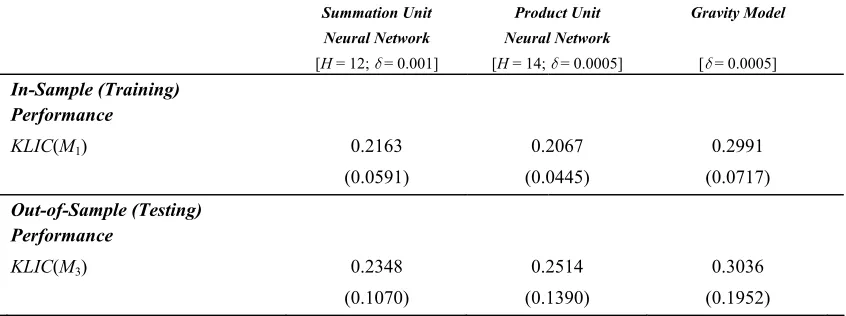
PLACE TABLE 2 ABOUT HERE

TABLE 2 summarizes the simulation results for the unconstrained neural network

models in comparison with the gravity model. Out-of-sample performance is measured

in terms of KLIC M

( )

3 . For matters of completeness, also training performance values

are displayed. The figures represent averages taken over 60 independent simulations

differing in the bootstrap samples and in the initial parameter values randomly chosen

from [-0.3, 0.3].

If out-of-sample [generalization] performance is more important than fast learning,

then the neural network models exhibit clear and statistically significant superiority. As

can be seen by comparing the KLIC-values the summation unit neural network model

ranks best, followed by the product unit model and the gravity model. The average

generalization performance, measured in terms of KLIC M

( )

₃ , is 0.2348 (H = 12),

compared to 0.2514 in the case of πΩ_L (H = 14), and 0.3036 in the case of τgrav

. These

differences in performance are statistically significant6. If, however, the goal is to

minimize execution time and a sacrifice in generalization accuracy is acceptable, then

the gravity model is the model of choice. The gravity model outperforms the neural

network models in terms of execution time, the summation unit network model by a

factor of 50 and the product unit network model by a factor of 30. But note that this is

mainly caused by two factors: first, that our implementations were done on a serial

platform even though the neural network models are parallelizeable, and, second, that

we implemented a rather time consuming termination criterion (κ =40, 000) to stop the

training process.

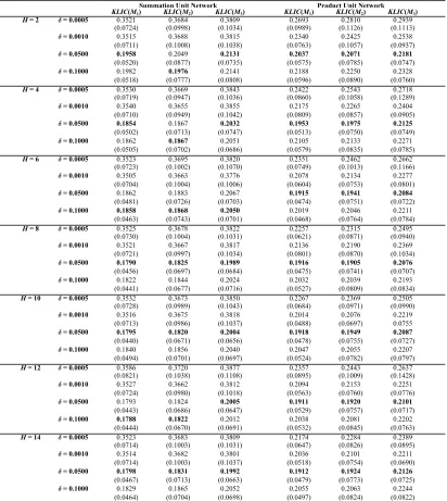
The Origin Constrained Case of Spatial Interactions: TABLE 3 presents some

and δ∈

{

0.0005, 0.0010, 0.0500, 0.1000

}

. Again some considerations are worth making.

First, a comparison with TABLE 1 illustrates that the consideration of a priori

information in form of origin constraints clearly improves the generalization

performance more or less dramatically. Second, the best result (averaged over the 60

independent simulation runs) in terms of average KLIC M

( )

3 was achieved with H = 8 and δ =0.0500 in both cases, the origin constrained summation unit neural network model ΣΩ₁OC, and the origin constrained product unit neural network model, πΩ₁OC.

Third, the summation unit model version slightly outperforms the product unit version.

Again this is primarily due to the logarithmic transformation of the input data in the

case of Σ OC 1

Ω . Fourth, model approximation improves as the complexity of the model grows with increasing H [up to H = 8, except H = 6 in the case of ΣΩ₁OC]. Fifth, there is

clear evidence that δ =0.0500 tends to lead to the best results (except H = 6 in the case

of ΣΩ₁OC), while δ =0.0005 tends to yield the poorest results, with only two

exceptions (H = 2 and 4) in the case of OC

1

Σ_{Ω . Sixth, there is strong evidence that the}

origin constrained neural network models are much less robust with respect to the

choice of the Alopex parameter δ in comparison to their unconstrained counterparts,

while the variability in prediction performance over changes in training, internal

validation and test samples, and parameter initialization is lower. Finally it is interesting

to note that forceful training encourages πΩ₁OC to produce the best generalization

ability in all cases considered.

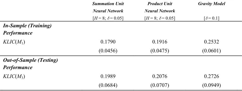
TABLE 4 reports the simulation results for the origin constrained neural network

models, ΣΩ₁OC and πΩ₁OC, in comparison with origτgrav. Training and generalization

performance are displayed. The figures represent again averages taken over 60

simulations differing in parameter initialization and bootstrap samples as in the other

tables. The modular summation unit neural network performs best, closely followed by

the product unit model version. Both outperform the gravity model predictions7. The

average out-of-sample performance of OC

1

Σ_{Ω with H = 8, measured in terms of}

( )

3

KLIC M , is 0.1989, compared to 0.2076 in the case of πΩ₁OC with H = 8, and 0.2726

in the case of origτgrav

. The gravity model would be the model of choice if the goal

would be to minimize execution time and a sacrifice in generalization would be

7. SUMMARY AND DIRECTIONS FOR FUTURE RESEARCH

In this contribution a modest attempt has been made to provide a unified framework for

neural spatial interaction modeling including the case of unconstrained and that of

origin constrained spatial interaction flows. We suggested and used a more suitable

estimation approach than available in literature, namely maximum likelihood estimation

under distributional assumptions of Poisson processes. In this way we could avoid the

weakness of least squares and normality assumptions that ignore the true integer nature

of the flows and approximate a discrete-valued process by an almost certainly

misrepresentative continuous distribution. Alopex, a powerful global search procedure,

was used to solve the maximum likelihood estimation problem.

Randomness enters in two ways in neural spatial interaction modeling: in the

splitting of the data into training, internal validation and test sets on the one side and in

choices about parameter initialization on the other. The paper suggests the

bootstrapping pairs approach to overcome this problem as well as the problem of scarce

data. In addition one receives a better statistical picture of the variability of the

out-of-sample performance of the models. The approach is attractive, but computationally

intensive. Each bootstrap iteration requires a run of the Alopex procedure on the

training bootstrap set. In very large real world problem contexts this computational

burden may become prohibitively large.

Although the discussion has been centered on several general families of neural

spatial interaction models, only one of the vast number of neural network architectures

and only one – even though powerful – estimation approach were considered. Thus, we

emphasize that our results are only a first step towards a more comprehensive

methodology for neural spatial interaction modeling. There are numerous important

areas for further investigation. Especially desirable is the design of a neural network

approach suited to deal with the doubly constrained case. Another area for further

research is greater automation of the cross-validation training approach to control

maximum model complexity by limiting the number of hidden units. Finding good

global optimization methods for solving the non-convex training problems is still an

important area for further research even though some relevant work can be found in

deserves further research activities to come up with methods that go beyond the current

rules of thumb. We hope that this paper will inspire others to pursue the investigation in

neural spatial interaction modeling further as we finally believe that this field is an

Endnotes

1

Sigmoid transfer functions such as the logistic function are somewhat better behaved than many other functions with respect to the smoothness of the error surface. They are well behaved outside of their local region in that they saturate and are constant at zero or one outside the training region. Sigmoidal units are roughly linear for small weights [net input near zero] and get increasingly nonlinear in their response as they approach their points of maximum curvature on either side of the midpoint.

2

Alopex is an acronym for algorithm for pattern extraction. 3

For the first two iterations, the weights are chosen randomly. 4

There is virtual unanimity of opinion that site specific variables, such as sj in this case, are generally

best represented as power functions. The specification of fij is consistent with general consensus that

the power function is more appropriate for analyzing longer distance interactions (Fotheringham and O’Kelly 1989).

5

In the case of the summation unit model versions the input data were preprocessed to logarithmically transformed data scaled into [0.1, 0.9].

6

assessed by means of the Wilcoxon-Test (comparison of two paired samples). The differences between ΩL and

grav

τ are statistically significant at the 1 % level (Z = -3.740, Sig. 0.000) as are the differences between L

π

Ω and τgrav (Z = -3.269, Sig. 0.001). But the differences between ΩL and L

π

Ω

are not statistically significant at the 1 % level (Z = -1.436, Sig. 0.151). 7

The differences between OC 1

Σ

Ω and origτgrav are statistically significant at the 1 % level (Z = -6.684, Sig. 0.000) as are the differences between OC

1

π

Ω and origτgrav (Z = -6.714, Sig. 0.000), while the differences between the neural network models are not statistically significant at the 1 % level (Z = -2.481, Sig. 0.130).

REFERENCES

Bergkvist, E. (2000). “Forecasting Interregional Freight Flows by Gravity Models.”

Jahrbuch für Regionalwissenschaft 20, 133-48.

Bergkvist, E. and L. Westin (1997). Estimation of Gravity Models by OLS Estimation,

NLS Estimation, Poisson and Neural Network Specifications. CERUM Regional

Dimensions, Working Paper No. 6.

Bia, A. (2000). A Study of Possible Improvements to the Alopex Training Algorithm.

In Proceedings of the VIth Brazilian Symposium on Neural Networks, pp. 125-130.

IEEE Computer Society Press.

Black, W.R. (1995). “Spatial Interaction Modelling Using Artificial Neural Networks.”

Journal of Transport Geography 3(3), 159-66.

Cover, T.M. (1965). “Geometrical and Statistical Properties of Systems of Linear

Inequalities with Applications in Pattern Recognition.” IEEE Transactions on

Electronic Computers 14, 326-34.

Efron B (1982). The Jackknife, the Bootstrap and Other Resampling Plans.

Philadelphia: Society for Industrial and Applied Mathematics.

Fischer, M.M. and S. Gopal (1994). “Artificial Neural Networks: A New Approach to

Modelling Interregional Telecommunication Flows.” Journal of Regional Science

34(4), 503-27.

Fischer, M.M. and Y. Leung (1998). “A Genetic-Algorithms Based Evolutionary

Computational Neural Network for Modelling Spatial Interaction Data.” The Annals

of Regional Science 32(3), 437-58.

Fischer, M.M. and Y. Leung (eds.) (2001). GeoComputational Modelling: Techniques

and Applications. Berlin, Heidelberg and New York: Springer.

Fischer, M.M. and M. Reismann (2000). Evaluating Neural Spatial Interaction

Modelling by Bootstrapping. Paper Presented at the 6th World Congress of the

Regional Science Association International, Lugano, Switzerland [accepted for

Fischer, M.M., K. Hlavackova-Schindler and M. Reismann (1999). “A Global Search

Procedure for Parameter Estimation in Neural Spatial Interaction Modelling.”

Papers in Regional Science 78, 119-34.

Fischer, M.M., M. Reismann and K. Hlavackova-Schindler (2001). Neural Network

Modelling of Constrained Spatial Interaction Flows, Paper Presented at the 41th

Congress of the European Regional Science Association, Zagreb, Croatia [accepted

for publication in the Journal of Regional Science].

Fotheringham, A.S. and M.E. O’Kelly (1989). Spatial Interaction Models:

Formulations and Applications. Dordrecht, Boston and London: Kluwer.

Giles, C. and T. Maxwell (1987). “Learning, Invariance, and Generalization in

High-Order Neural Networks.” Applied Optics 26(23), 4972-8.

Gopal, S. and M.M. Fischer (1993). Neural Net Based Interregional Telephone Traffic

Models. In Proceedings of the International Joint Conference on Neural Networks

IJCNN 93 Nagoya, Japan, October 25-29, pp. 2041-4.

Gopal, S. and M.M. Fischer (1996). “Learning in Single Hidden-Layer Feedforward

Network Models: Backpropagation in a Spatial Interaction Context.” Geographical

Analysis 28(1), 38-55.

Kullback, S. and R.A. Leibler (1951). “On Information and Sufficiency.” Annals of

Mathematical Statistics 22, 78-86.

Longley, P.A., S.M. Brocks, R. McDonnell and B. MacMillan (eds.) (1998).

Geocomputation: A Primer. Chichester: John Wiley.

Mozolin, M., J.-C. Thill and E.L. Usery (2000). “Trip Distribution Forecasting with

Multilayer Perceptron Neural Networks: A Critical Evaluation.” Transportation

Research B 34, 53-73.

Nijkamp, P., A. Reggiani and T. Tritapepe (1996). Modelling Intra-Urban Transport

Flows in Italy. TRACE Discussion Papers TI 96-60/5, Tinbergen Institute, The

Netherlands.

Openshaw, S. (1993). “Modelling Spatial Interaction Using a Neural Net.” In

Geographic Information Systems, Spatial Modeling, and Policy Evaluation, edited

by M.M. Fischer and P. Nijkamp, pp. 147-64. Berlin, Heidelberg and New York:

Press, W.H., S.A. Teukolsky, W.T. Vetterling and B.P. Flannery (1992). Numerical

Recipes in C: The Art of Scientific Computing. Cambridge: University Press.

Reggiani, A. and T. Tritapepe (2000). “Neural Networks and Logit Models Applied to

Commuters’ Mobility in the Metropolitan Area of Milan.” In Neural Networks in

Transport Applications, edited by V. Himanen, P. Nijkamp and A. Reggiani, pp.

111-29. Aldershot: Ashgate.

Rumelhart, D.E., R. Durbin R., R. Golden and Y. Chauvin (1995). “Backpropagation:

The Basic Theory.” In Backpropagation: Theory, Architectures and Applications,

edited by Y. Chauvin and D.E. Rumelhart, pp. 1-34. Hillsdale [NJ]: Lawrence

Erlbaum Associates.

Thill, J.-C. and M. Mozolin (2000). ”Feedforward Neural Networks for Spatial

Interaction: Are they Trustworthy Forecasting Tools?” In Spatial Economic Science:

New Frontiers in Theory and Methodology, edited by A. Reggiani, pp. 355-81.

Berlin, Heidelberg and New York: Springer.

Young, T.Y. and T.W. Calvert (1974). Classification, Estimation and Pattern

List of Figures:

FIG. 1. Architecture of the Unconstrained Summation Unit Neural Spatial Interaction Models as Defined by Equation (1) for N = 3

FIG. 2. Architecture of the Unconstrained Product Unit Neural Spatial Interaction Models as Defined by Equation (3) for N = 3