Two Stage Wavelet based Image Denoising
Glincy Abraham, Neethu Mohan, Sreekala S, Neethu Prasannan, K P Soman
Centre for Excellence in Computational Engineering and Networking Amrita Vishwa Vidyapeetham, Coimbatore, Tamil Nadu, India-641112
ABSTRACT
In this paper we are proposing a 2-stage wavelet based denoising technique. First stage of denoising is performed on the approximation coefficient obtained from the level 1 wavelet decomposition [1] of the noisy image and second stage of denoising is applied on the reconstructed image. The second stage denoising has shown a better result on to the reconstructed image. The detail coefficients are newly estimated from the first level denoised approximation coefficients. For denoising, techniques like Total Variation [3], Split Bregman [4] and NL means [5] are used. The quality of results obtained from different denoising techniques has been measured using various objective matrices such as PSNR, MSE on standard test images.
General Terms
Denoising, Wavelet decomposition
Keywords
Total Variation, Split-Bregman, NL-means, Edge detection
1.
INTRODUCTION
Denoising is an important preprocessing technique in image processing, which removes the noise while preserving the image quality [8]. In order to retain the edge information and to maintain the quality of the denoised image, wavelet based decomposition [9] was introduced along with conventional image denoising [2]. For estimating the performance of this technique various wavelets and denoising techniques are applied on the standard images.
Nowadays Wavelet transforms has become a powerful computational tool and plays a significant role in image processing. DWT (Discrete Wavelet Transform) decomposes the input image into approximation and detail coefficients. In this paper, we applied the denoising techniques on these approximation coefficients and these denoised coefficients are used for the estimation of new detail coefficients (horizontal, vertical and diagonal). The denoised approximation and estimated detail coefficients are used for the reconstruction of the image. Amount of noise in this reconstructed image will be considerably less. Second stage denoising helps in further filtering of noises in the image and is shown in section 4. This estimation is done with different wavelets such as ‘haar’, ‘db2’, ‘bior2.4’.
The techniques used in this paper for denoising include TV denoising [3] Split-Bregman [4] and NL-Means [5]. TV denoising is very effective denoising technique which removes the noise by solving a nonlinear minimization equation. Split Bregman is one of the fastest algorithms for solving through convex optimization. NL-means is another denoising technique based on non-local averaging of pixels. For efficient edge detection Canny [6] method proposed by John F Canny is used, which uses multi-stage algorithm.
Canny uses thresholding withhysteresis which requires two thresholds – high and low.
Section 2 gives an over view of various denoising techniques. Section 3 introduces the proposed method. Section 4 discusses the results for various inputs and its quality measurements.
2.
DENOISING TECHNIQUES
2.1
Total Variation
Total variation based filtering was introduced by Rudin, Osher, and Fatemi [3]. Total variation denoising is applicable in many digital images processing for reducing the noise. The total variation (TV) of a signal measures how much the signal changes between signal values. Total variation of an N point signal
X n
( ),1
n
N
is defined as2
( )
( )
(
1)
N
n
TV x
x n
x n
(1)For an image
u x y
( , )
, then TV to be defined as,1 1 1 1 1 1 1 1
( )
( , )
(
1, )
( , )
( ,
1)
( ,
)
(
1,
)
(
, )
(
,
1)
(2)
M N i j M i M j
TV u
u i j
u i
j
u i j
u i j
u i N
u i
N
u M j
u M j
The objective function for total variation can be defined as
2 2 2 2
0
(
)
(3)
y x
t
x y x y
u
u
u
x
u
u
y
u
u
u u
Where λ is the regularization parameter, which controls how much smoothing is done. For higher values of λ denoised image is very similar to original noisy image. If it is too small value edge information cannot preserve, so we have to choose an optimum value for λ.
2.2
Split-Bregman
Split-Bregman is a suitable technique for solving total variation minimization problem based on partial differential equations. Optimization problems of the following type can be solved by using Split-Bregman technique
, 1 2
min
u X v R v
H u
( ) ( / 2)
d
( )
u
(5)
Then the simplified form of Split Bregman can be given as
1 1
,
2 2
(
,
)
min
( , )
(
,
)
,
,
/ 2
( )
(6)
k k k k
u X d R
k k k k
u u
u
d
J u d
J u d
b
b d
d
d
u
2, 2 2
( k, k) min ( , ) ( / 2) ( ) k (7)
u X d R
u d J u d
d
u b CWhere
C
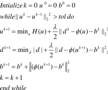
2 is a constant.Split-Bregman Algorithm [7]
0 0
1 2 2
1 2
2
1 1 2
2 2
1 1
2
0
0
0
||
||
min
( )
||
( )
||
2
min |
|
||
(
)
||
2
( (
)
k k
k k k
u
k k k
d
k k k k
Intialize k
u
b
while u
u
tol do
u
H u
d
u
b
d
d
d
u
b
b
b
u
b
1
k
k
end while
2.3
Non Local Means Algorithms
It is one of the denoising techniques based on non local averaging of all the pixels in the image. Noise contains both high and low frequency components. Earlier techniques focus on removing the high frequency noise at the cost of high frequency fine details of the original image. These techniques take least care in removing the low frequency noises. Non-local means is an algorithm that takes care of the loss of details.
The non local means algorithm considers the extensive amount of self similarity of pixels in an image[10]. Figure 1 [5] explains the self similarity of pixels in an image. Consider the pixel-points p, q1 and q2 and their respective neighborhood
points. The neighborhoods of pixel p and q1 are similar but
that of q2 are not similar, which means most pixels in same
[image:2.595.333.521.70.197.2]columns of p will have similar neighborhood as that of p. Pixels with similar neighborhoods can be used to denoised an image. The weighted intensity average of pixels with similar value provides the new denoised value.
Fig 1. Example of self similarity in an image
The continuous version of NLM can be written as ( , ) ( )
( ) (8)
( , )
o
w x y u y dy
u x
w x y dy
Where
u
0:
R
is the given noisy image,:
u
R
is the outcome of the NLM algorithm, functionw
is defined as
2 2
( ) ( ) ( ) /
,
,
a o o
G z u x z u y z dz h
w x y
e
Where2
( ) o( ) o( )
a
G z u x z u y z dz is the distance between patches located at
x y
,
.h
is positive constant which acts as scale parameter.Ga
is Gaussian function with standard deviationa
.3.
PROPOSED METHOD
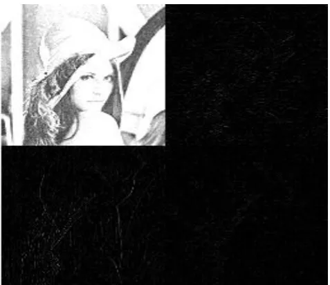
[image:2.595.56.245.320.477.2]Fig 2: Approximation and detailed coefficient obtained by using DWT.
Fig 3:
Block diagram of the proposed methodNew Detail Coefficients
Stage 2 Denoising
Denoised Image
IDWT
EdgeDet
ecti
on
EdgeDete
ction
Edge
Detec
tion
VerticalDiffer
encing
Horizontal
Differen
cing
DiagonalDifferen
cing
Stage 1 Denoising CA CH CV CD
Noisy Image
[image:4.595.113.501.71.201.2]
(a)
(b) (c) (d)
Fig 4. The performance of the proposed algorithm for lena image with SNR of 25 dB a)original image b) noisy image c)first stage denoised image d)second stage denoised image. Bregaman denoising and bior2.4 wavelet is used
4.
RESULTS AND DISCUSSION
For doing experiment Matlab 2009 is been used. Proposed method uses three different wavelets such as ‘haar’, ‘db2’, ‘bior2.4’ and different standard images (clean images) such as ‘lena’, ‘cortex’, and ‘pepper’. The clean images used are shown in figure. Additive white gaussian noise are added to these clean images with varying SNR (Signal to Noise Ratio)
levels such as 10dB, 15dB, 20dB, 25dB, 30dB and 35dB. The result obtained by using Total variation, NL- means and Split Bregman are shown below with the help of figures, tables. The metrics used to evaluate the method are PSNR (Peak-Signal-to-Noise ratio) and MSE (Mean Square Error). The SNR level for the figure is 25dB. The four images in each figure represents original image, noise added image, first stage denoised image and second stage denoised image.
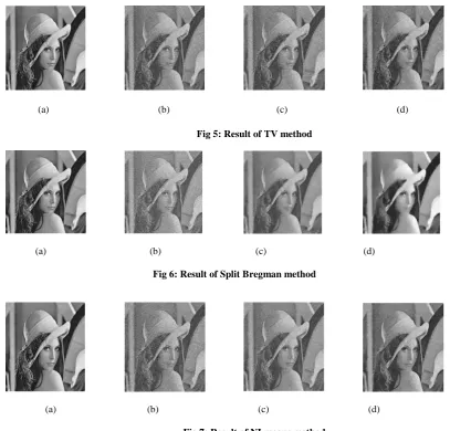
(a) (b) (c) (d) Fig 5: Result of TV method
(a) (b) (c) (d) Fig 6: Result of Split Bregman method
[image:4.595.85.493.347.737.2](a) (b) (c) (d) Fig 8: Result of TV method
(a) (b) (c) (d) Fig9: Result of Split Bregman method
(a) (b) (c) (d) Fig10: Result of NLmeans method
(a) (b) (c) (d) Fig11: Result of TV method
(a) (b) (c) (d) Fig13: Result of NLmeans method
Outputs obtained by applying three denoising techniques in different images with SNR 25db and Bior2.4 wavelet. a) Original image b)Noisy image c)First Level Denoised Image d) Second Level Denoised Image
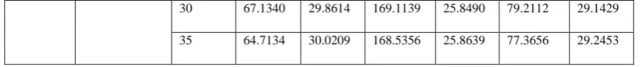
Table1: PSNR and MSE values for various SNR , denoising technique and wavelets applied on different images
IMAGES WAVELETS SNR
TV SPLIT-BREGMAN NL-MEANS
MSE PSNR MSE PSNR MSE PSNR
LENA
Haar
10 469.6815 21.4128 192.7240 25.2814 414.0674 21.9601 15 307.8095 23.2480 184.3603 25.4741 269.3889 23.8270 20 229.4304 24.5243 180.6849 25.5616 208.9667 24.9300 25 190.0711 25.3416 183.4872 25.4947 167.4253 25.8926 30 166.3524 25.9205 180.0933 25.5758 146.0011 26.4872 35 149.5035 26.3843 180.2803 25.5713 133.4379 26.8780
Bior2.4
10 482.4780 21.2960 171.8085 25.7804 476.3154 21.3519 15 306.2128 23.2706 158.4206 26.1327 291.7184 23.4812 20 225.1808 24.6055 151.7401 26.3198 210.5647 24.8969 25 175.1624 25.6964 150.7249 26.3490 164.7860 25.9616 30 148.2276 26.4215 154.5793 26.2393 141.2835 26.6299 35 125.4892 27.1447 153.1577 26.2794 119.9662 27.3402
Db2
PEPPER
Haar 25 157.3129 26.1632 166.3207 25.9213 146.7435 26.4652 30 140.4432 26.6558 167.3562 25.8944 130.7190 26.9674 35 128.8912 27.0286 165.4439 25.9443 121.6589 27.2794
Bior2.4
10 357.5616 22.5973 146.2815 26.4789 361.8132 22.5460 15 220.0797 24.7050 137.0415 26.7623 219.8704 24.7091 20 161.1183 26.0594 129.8188 26.9974 156.9398 26.1735 25 126.8048 27.0994 131.9146 26.9279 125.2639 27.1525 30 106.5310 27.8560 130.1494 26.9864 109.3381 27.7431 35 94.4527 28.3787 130.5413 26.9733 96.3602 28.2918
Db2
10 329.8899 22.9471 153.3561 26.2738 319.2815 23.0891 15 205.4821 25.0031 148.6414 26.4094 194.5471 25.2406 20 151.1988 26.3353 142.5305 26.5917 143.5987 26.5593 25 122.8566 27.2368 141.7675 26.6150 119.6524 27.3516 30 105.1201 27.9139 143.8016 26.5532 103.5709 27.9784 35 93.5434 28.4207 141.4719 26.6241 92.9523 28.4482
CORTEX Haar
10 173.4387 25.7393 192.8844 25.2778 171.4136 25.7904 15 133.0572 26.8904 192.7704 25.2804 133.3394 26.8812 20 117.0054 27.4487 194.0108 25.2525 122.7949 27.2390 25 106.4295 27.8602 191.7412 25.3036 114.7209 27.5344 30 101.8293 28.0521 192.4496 25.2876 111.4165 27.6613 35 96.9273 28.2663 191.6156 25.3065 107.9106 27.8002
Bior2.4
10 147.0779 26.4553 151.4136 26.3292 157.2083 26.1660 15 99.9823 28.1316 151.6972 26.3210 107.4039 27.8206 20 80.6164 29.0965 151.9697 26.3132 91.4771 28.5177 25 69.7430 29.6958 152.6894 26.2927 82.1508 28.9847 30 64.9670 30.0039 152.8228 26.2889 77.4640 29.2398 35 58.6304 30.4496 152.46 26.2992 72.8118 29.5088
Db2
5.
CONCLUSION
[image:8.595.74.524.72.119.2]In this paper, a two stage wavelet based denoising method is presented. Experiments are conducted on 3 different images with different SNR values and the results for various denoising techniques are compared. The proposed method gives good results for different SNR values as seen in the table. Db2 and Bior2.4 wavelet gives better results compared with Haar. Here in denoising, only the detailed coefficients obtained from the dwt are retained, keeping the rest of the coefficients as zero. In future, denoised versions of these coefficients could also be utilized to provide better result.
6.
REFERENCES
[1] Stephane G Mallat “A theory for multiresolution signal decomposition:The wavelet representation”IEEE Transactions On Pattern Analysis And Machine Intelligence,Vol 11, No. 7. July 1989
[2] Nilamani Bhoi, Dr. Sukadev Meher” Total Variation based Wavelet Domain Filter for Image Denoising” First International Conference on Emerging Trends in Engineering and Technology
[3] L. Rudin, S. Osher, and E. Fatemi. Nonlinear total variation based noise removal algorithms. PhysicaD, 60:259–268, 1992
[4] Jacqueline Bush “Bregman Algorithms” Senior Thesis. University of California, Santa Barbara, June 10, 2011 [5] A.Buades, B.Coll, and J Morel “A non-local algorithm
for image denoising”, IEEE International Conference on Computer vision and Pattern Recognition,2005
[6] John Canny, member, IEEE, “A Computational Approach to Edge Detection”, IEEE Transactions on Pattern Analysis and Machine Intelligence, VOL. PAMI-8, NO. 6, November 1986
[7] Bregman Algorithms Author: JacquelineBush Supervisor Dr.CarlosGarc´ıa-Cervera June 10, 2011 [8] R C.Gonzalez and R.E Woods,Digital Image Processing,
Addison Wesley Longman Inc.,2000.
[9] Kossi Edoh and John Paul Roop “A Fast Wavelet Multilevel Approach to Total Variation Image Denoising”, International Journal of Signal Processing, Image Processing and Pattern Recognition Vol. 2, No.3,September 2009.