Ratio Cum Product Estimator Using Multiple Auxiliary Attributes in Two Phase Sampling

http://dx.doi.org/10.4236/ojs.2014.44024

Ratio-Cum-Product Estimator Using Multiple

Auxiliary Attributes in Two-Phase Sampling

John Kung’u, Leo Odongo

Department of Mathematics, Kenyatta University, Nairobi, Kenya Email: [email protected]

Received 21 March 2014; revised 21 April 2014; accepted 28 April 2014

Copyright © 2014 by authors and Scientific Research Publishing Inc.

This work is licensed under the Creative Commons Attribution International License (CC BY).

http://creativecommons.org/licenses/by/4.0/

Abstract

In this paper, we have proposed three classes of ratio-cum-product estimators for estimating pop- ulation mean of study variable for two-phase sampling using multi-auxiliary attributes for full in-formation, partial information and no information cases. The expressions for mean square errors are derived. An empirical study is given to compare the performance of the estimator with the ex-isting estimator that utilizes auxiliary attribute or multiple auxiliary attributes. The ra-tio-cum-product estimator in two-phase sampling for full information case has been found to be more efficient than existing estimators and also ratio-cum-product estimator in two-phase sam- pling for both partial and no information case. Finally, ratio-cum-product estimator in two-phase sampling for partial information case has been found to be more efficient than ratio-cum-product estimator in two-phase sampling for no information case.

Keywords

Ratio-Cum-Product Estimator, Multiple Auxiliary Attributes, Two-Phase Sampling and Bi-Serial Correlation Coefficient

1. Introduction

The use of supplementary information is a widely discussed issue in sampling theory. Auxiliary variables are commonly used in sample survey practices to obtain improved designs and to achieve higher precision in the es- timates of some population parameters such as the mean or the variance of a study variable. The concept of ratio estimation was introduced in sample survey by Cochran [1]. It is preferred when the study variable is highly po- sitively correlated with the auxiliary variable. Murthy [2] proposed the product estimator for negatively corre- lated study variable(s) and auxiliary variable which was similar to ratio estimator.

sitively correlated with the variable under study, using a linear combination of ratio estimator based on each auxiliary variable. Raj [4] suggested a method of using multi-auxiliary information in sample survey. Using this idea, Singh [5] proposed a multivariate expression of product estimator where the study variable was negatively correlated with the multi-auxiliary variable. In the same year, Singh [6] proposed a ratio-cum-product estimator and its multi-variable expression. Singh and Tailor [7] proposed a ratio-cum-product estimator for finite popula-tion mean in simple random sampling using coefficient of variapopula-tion and coefficient of kurtosis which was more efficient than the previous ratio-cum product estimator.

Jhajj, Sharma and Grover [8] proposed a general family of estimators using information on auxiliary attribute. They used known information of population proportion possessing an attribute (highly correlated with study va- riable Y). The attribute are normally used when the auxiliary variables are not available, e.g. amount of milk produced, a particular breed of cow or amount of yield of wheat and a particular variety of wheat. Bahland Tu- teja [9] proposed ratio and product type exponential estimators using auxiliary attribute. Rajesh, Pankaj, Nirmala and Florentins [10] used the information on auxiliary attribute in ratio estimator in estimating population mean of the variable of interest using known attributes such as coefficient of variation, coefficient kurtosis and point biserial correlation coefficient. The estimator performed better than the usual sample mean and Naikand Gupta [8] estimator. Rajesh, Pankaj, Nirmala and Florentins [10] also used the auxiliary attributes in ratio-product type exponential estimator following the work of Bahland Tuteja [9], the estimator was more efficient compared to mean per unit, ratio and product type exponential estimators as well as Naik and Gupta [11] estimator.

The concept of double sampling was first proposed by Neyman [12] in sampling human populations when the mean of auxiliary variable(s) was unknown. It was later extended to multiphase by Robson [13]. It is advanta- geous when the gain in precision is substantial as compared to the increase in the cost due to collection of in- formation on the auxiliary variable for large samples. In most survey, the auxiliary information is always availa- ble and every form of auxiliary information should be used in developing sampling strategies. Samiuddinand Hanif [14] introduced the following approach of using auxiliary variable.

1) Full information case: Information for all auxiliary variables is available 2) No information case: Information for all auxiliary variables is not available.

3) Partial information case: Information for some auxiliary variable is available for all population units. We have used these strategies to develop ratio-cum-product estimators using multiple auxiliary attributes for full information, partial and no information cases.

Hanif, Haq and Shahbaz [15] proposed a general family of estimators using multiple auxiliary attribute in sin- gle and double phase sampling. The estimators had a smaller MSE compared to that of Jhajj, Sharma and Grov- er [8]. They also extended their work to ratio, product and regression estimators which were generalization of Naik and Gupta [11] estimator in single and double phase sampling with full information, partial information and no information.

The concept of multiple auxiliary attributes was proposed by Hanif, Haq and Shahbaz [16], and then extended to ratio and product estimators. In this paper, we have incorporated the multiple auxiliary attributes in ratio- cum-product estimator in two-phase sampling as proposed by Singh [7] and used strategies introduced by Sa-miuddinand Hanif [14] and also incorporate Arora and Bansi [17] approach in writing down the mean squared error.

2. Preliminaries and Notations

2.1. Notations

Consider a population of N units. Let Y be the variable for which we want to estimate the population mean and

1, 2, , q

P P  P are q auxiliary attributes. For two-phase sampling design, let n₁ and n₂

(

n2 <n1

)

be sample

sizes for first and second phase respectively. In defining the attributes we assume complete dichotomy so that

1, if unit of population possess auxiliary attribute

0, otherwise

th th

ij

i j

τ =  

Let

1

N j ij

i

A

τ

=

=

∑

and

1

n j ij

i

a

τ

=

sessing attribute

τ

_j. Let P_j Aj N

= and p_{j( )2} aj n

= be the corresponding proportion of units possessing a specific attributes

τ

_j and y is the mean of the main variable at second phase. Let pj( )1 and pj( )2 denote the jth

auxiliary attribute form first and second phase samples respectively and y₂ denote the variable of interest from second phase. Let P_j and Cpj denote the population means and coefficient of variation of

th

j auxiliary attribute respectively and

ρ

Pbj denotes the population bi-serial correlation coefficient of Y and Pj. Let pj( )1

be proportion of units possessing attribute r_j in first phase sample of size n₁ while pj( )2 be proportion of units

possessing attribute r_j in second phase sample of size n₂. Further, let

1 1

1 1

n N

θ =_ − _

  2 2

1 1

n N

θ =_ − _

 

(

θ2 <θ1

)

2 2 y

e =y −Y ,

( )1 ( )1

j j j

e_τ = p −P, e_{τ( )2} = p_{j( )2} −P_j j=

(

1, 2,,q

)

(1.0) where ey₂, eτj( )1 and eτj( )2 are sampling error which are assumed to be very small. We let

j j

j

p v

P

= , 1 1

j

j i

j r

j j

p P

v e

P P

−

− = = , 1 1

j

j r

j

v e

P

= + (1.1)

while ( )

( )

2

1

j jd

j

p v

p

= , ( )

( )

( ) ( ) ( )

2 2 1

1 1

1 j 1 j j

jd

j j

p p p

v

P P

−

− = − =

( ) ( )

( )

( ) ( )

(

2 1

)

( )

2 1 1

1

1

1 j j j j 1 j

j

r r

r r r

jd

j r j j

e e

e e e

v

P e P P

− −

−  

 

− = = +

 

+ _{ } (1.2)

Here we shall take

(

vjd −1

)

to, term of order 1

n as

( ) ( )

(

1 2

)

₍

₎

1 r j r j for 1, 2, ,

jd

j

e e

v j q

P

−

≈ − =  (1.3)

Let 2

2 2

2

y y

S C

Y

= and

2

2 i

j j

S C

P

τ

τ = are the coefficient of variation of study variable and the auxiliary variables

respectively. The bi-serial correlation coefficient between study variable and auxiliary attributes is given by

j j

j y Pb

y

S

S S

τ

τ

ρ = . Then for simple random sampling without replacement for both first and second phases we write

by using phase wise operation of expectations as:

( )

( )

( )

(

( )

)

( )

(

( ) ( )

)

(

)

(

)

(

_{( ) ( )}

)

(

)

( )

(

( ) ( )

)

(

)

(

)

(

_{( )}

(

_{( ) ( )}

)

)

(

)

(

)

( ) ( )

(

)

2 2 2 2 2 2

2 1 2 2 2

2 1 2 2 1 2

1 2

2 2

2 2 2 2 2

2 2 2

1 2 2

2 2

1 2 1 2

2

2

, ,

,

, ;

j j j

i J

i i i j i j

i i i i

j j i i

j j j j j j

j j

y y i y j y Pb

y j y y i j

j i j

E e Y C E e P C E e e YP C C

E e e e YP C C E e e P P C C i j

E e e e X C E e e e P P C C i j

E e e

τ τ τ τ

τ τ τ τ τ τ τ τ τ τ

τ τ τ τ τ τ τ τ τ ττ

τ τ

θ θ θ ρ

θ θ ρ θ ρ

θ θ θ θ ρ

θ

= = =

− = − = ≠

− = − − = − ≠

− =

(

−

)

( ) ( )

(

)

(

( ) ( )

)

(

_{1 2 1 2}

)

(

)

(

)

2 2

1 P Cj τj, E eτi eτi eτj eτj 2 1 P P C Ci j τj τi τ τj i; i j

θ − − = θ θ− ρ ≠

(1.4)

If A is a square matrix, its inverse can be written using ad joint matrix as,

( )

( )

1 1 T

ij

Adj A

A C

A A

(

2

)

.

1

p

p p

y

y

R

R

τ

τ τ

ρ

= −



 

Arora and Lai [1] (1.6)

The following notations will be used in deriving the mean square errors of proposed estimators

p y

R _τ 

Determinant of population correlation matrix of attributes y, ,

τ τ

_{1 2},,

τ

_q−1 and

τ

_q.

j p

y y

R_τ

τ



Determinant of jth minor of

q y

R _τ 

corresponding to the jth element of

j Pb

ρ .

2

r Pb

ρ Denotes the multiple coefficient of determination of y on τ τ₁, ₂,,τr−₁ and τr.

2

r Pb

ρ Denotes the multiple coefficient of determination of y on y, ,

τ τ

_{1 2},,

τ

q−₁ and

τ

q.

r

R_τ 

Determinant of population correlation matrix of attributes τ τ₁, ₂,,τr−₁ and τr.

i r y

R _τ 

Determinant of the correlation matrix of yi, ,τ τ_{1 2},,τr−₁ and τr.

.

i q y

R _τ 

Determinant of the correlation matrix of y_i, ,

τ τ

_{1 2},,

τ

_q−1 and

τ

_q.

. .

i j r y y

R _τ



Determinant of the minor corresponding to

ij Pb

ρ

of the correlation matrix of

(

)

1 2 1

, , , , , and

i j r r

y y τ τ τ ₋ τ i≠ j .

. .

i j q y y

R _τ



Determinant of the minor corresponding to

ij Pb

ρ

of the correlation matrix

(

)

1 2 1

, , , , , and .

i j q q

y y τ τ τ ₋ τ i≠ j (1.7)

2.2. Mean per Unit in Two-Phase Sampling

The sample mean y₂ using simple random sampling without replacement is given by, 2

2 1 2

1 n i i

y y

n =

=

∑

(1.8) While the variance of y₂ is given by,

( )

2 2

2 2 y

V y =Y

θ

C (1.9)

2.3. Ratio and Product Estimator in Two-Phase Sampling Using One Auxiliary Attributes

In order to have an estimate of the population mean Y of the study variable y, assuming the knowledge of the population proportion P, Naik and Gupta [8] defined ratio and product estimators of population mean when the prior information of population proportion of units possessing the same attribute is variable. Naik and Gupta [8]

proposed the following estimators:

( )

1

2 1 2

2

R

P

t y

p

α

 

= _{ }

  (1.10)

( )

2

2 2 1 2

P

p

t y

P

α

 

= _{ }

  (1.11)

The MSE of t_{R1 2( )} and t_{P1 2( )} up to the first order of approximation are given respectively by,

( )

( )

2

(

2 2 2

)

2 1 1

1 2 y P 2 P y Pb P

MSE t =θY C +α C − αC C ρ (1.12)

( )

( )

(

2

)

2 2 2 2

2 2 2

1 2 y P 2 P y Pb P

MSE t =θY C +α C + α C C ρ (1.13)

The optimum value are 2

1

y Pb

r

C

C

ρ

α = and 2

2

y Pb

r

C

C

ρ

2.3. Ratio and Product Estimator Using Multiple Auxiliary Attributes in Two-Phase

Sampling

The ratio and product estimators by Hanif, Haq and Shahbaz [5] for single phase sampling using information on multiple auxiliary attributes are given respectively by,

( )

( ) ( ) ( )

1 2

1 2 2

2 2

2 1 2 2 2

q

q R

q

P

P P

t y

p p p

β β β

     

     

=

     

     

(1.13)

( ) ( ) ( ) ( )

1 2

2 1 2 2 2 2

2 2

1 2

j

k

P

k

p p p

t y

P P P

α α α

     

= _  _{ } _ _ _

      (1.14) The MSE of the t_{R2 2( )} and t_{P2 2( )} up to the first order of approximation are given respectively by,

( )

( )

2 2

(

2

)

2

2 2 y 1 Pbq

R

MSE t =θY C −ρ _τ

 (1.15)

( )

( )

2 2

(

2

)

2

2 2 y 1 Pbq

P

MSE t =θY C −ρ _τ

 (1.16)

3. Methodology

3.1. Ratio-Cum-Product Estimator Using Multiple Auxiliary Attributes for Full

Information Case in Two-Phase Sampling

If we estimate a study variable when information on all auxiliary variables is available from population, it is uti- lized in the form of their means. By taking the advantage of ratio-cum-product technique for two-phase sam- pling, a generalized estimator for estimating population mean of study variable Y with the use of multi auxiliary attributes is proposed as:

( )

( ) ( ) ( )

( ) ( ) ( )

1 2 1 2

2 1 2 2 2 1 2

2 3.1

1 2

2 1 2 2 2

k k k q

k k q

k RP

k k q

k

p p p

P

P P

t y

p p p P P P

α α α β+ β+ β

+ +

+ +

           

     

= _{     } _ _ _ _{ }

      

      

(3.1)

Using (1.0), (1.1) in (3.1) and ignoring the second and higher terms for each expansion of product and after simplification, we write,

( )3.1 2 ( )2 ( )2

1 j 1 j j

h k q k

j r r

RP

j j j k j

Y Y

t y e e

P P

α + = β

= = +

= −

∑

+

∑

(3.2)

The mean squared error of ratio-cum-product estimator is:

( )

(

)

2 ( )2 ( )2

2 2

3.1

1 j 1 j j

h k q k

y j r r

RP

j j j k j

Y Y

MSE t E e e e

P P

α + = β

= = +

 

= _ − + _



∑

∑

 (3.3)

We differentiate Equation (3.3) partially with respect to αi

(

i=1, 2,,k

)

and βi

(

i= +k 1,k+2,,p

)

then equate to zero, using (1.5), (1.7) and (1.4), we get

( )

1

1 _j

p j

p

j y

j y

j

C R R_τ C P_τ τ τ

α +

= −





(3.4)

( )

1

1 _j

q i

q

j y

j y

j

C R R C P_τ τ τ

τ

β +

= − −

 

(3.5)

( )

(

)

( )2 ( )2

2 2

3.1

1 1

j h k q j

k

y y j j

RP

j j j k j

e e

MSE t E e e Y Y

P P

τ τ

α + = β

= = +       = _ − + _  _{ } 

∑

∑

 (3.6)

Using (1.4) in (3.6), we get,

( ) 2 2

2 2

2 3.1

1 1

( ) _{j j j j}

k h q k

y j j y Pb j j y Pb

RP

j j

MSE t θY C α P C C_τ ρ β P C C_τ ρ

+ =

= =

 

= _ − + _



∑

∑

 (3.7)

Using the optimum value

α

_j and

β

_j in (3.4) and (3.5) and (3.7), we get,

( )

(

)

2 2

( )

2

( )

2

2 3.1 1 1 1 1 j j q q

j j j j

j q j q

y k h q y

k

j y j y

y j y Pb j y Pb

RP

j j j k j

R R

C C

MSE t Y C P C C P C C

P C R P C R

τ _τ τ _τ

τ τ

τ τ τ τ

θ ρ + = ρ

= = +     = _ + − + − _    

∑



∑

   (3.8) Or ( )

(

)

2 2 2

( )

3.1

1

1 _{j j}

q _q q q j y y Pb RP y j Y C

MSE t R R

R τ τ τ

τ θ ρ =   = _ + − _  

∑

_   (3.9) Or ( )

(

)

2 2

2 3.1 q q y y RP R

MSE t Y C

R τ τ θ =   (3.11)

Using (1.6) in (3.11), we get,

( )

(

)

2

2 2

3.1 2 .

( ) 1

q

RP y y Pb MSE t =θ Y C −ρ _τ



(3.12)

3.2. Ratio-Cum-Product Estimator Using Multiple Auxiliary Attributes for Partial

Information Case in Two-Phase Sampling

In this section, we proposed a ratio-cum-product estimator using multiple auxiliary attributes for partial infor- mation case in two-phase sampling using k auxiliary attributes with “s” known and “k− s” unknown attributes which are positively correlated with study variable Y and g− k auxiliary attributes with “g− t” known and “g− k +

t” unknown attributes which are negatively correlated with study variable (Y). The proposed ratio-cum-product estimator for partial information case is as follows,

( ) ( ) ( ) ( ) ( ) ( ) ( ) ( ) ( ) ( ) ( ) ( ) ( ) ( ) ( ) ( ) ( ) ( )

1 1 2 2

1 2 1

1 1 ₁ 2 1 ₂ 1

2 3.2

1 2 1 2 2 2 2 2 2 2

1 1 2 1 1 1 2

1 2 2 2 2 1 1

r r

r r k k

s _s

RP

r r

s s k k k

r r k k

p _P p _P p _P

t y

p p p p p p

p p p p p

p p P p

α β α β α β

α+ α+ α γ+

+ + + + + +                         =                                         ⋅                   ( ) ( ) ( ) ( ) ( ) ( ) ( ) ( ) ( ) ( ) ( ) ( ) ( ) 2 1 1 2 2

1 2 2 2

1 2 1

2 2 2 2 1 2 2 2 2

2 1 1 1 2 1 1

k k

h h h g

k h

k

k k

g

k h h h h

k h h h h g

p

P p

p p p p p p

P p P p p p

γ λ

γ γ γ γ

λ λ + + + + + + + + + + + + + + +                                     ⋅_ _{  } _ _{      }             (3.13)

Using (1.0), (1.1) in (3.13) and ignoring the second and higher terms for each expansion of product and after simplification, we write,

( )

(

( ) ( )

)

( )

(

( ) ( )

)

( ) ( )

(

)

( )

(

( ) ( )

)

1 2 2 1 2

1 2 2 1 2

2 3.2

1 1 1

1 1 1

j ij j j ij

j ij j j ij

r r k

r r r r r

RP

j j j j j r j

g

t k h t k h

r r r r r

j k j i k j i k h j

Y Y Y

t y e e e e e

P P P

Y Y Y

e e e e e

P P P

= = = + + = + = = + = + = + + = + − − + − − − + − −

∑

∑

∑

Mean squared error of t_{RP( )3.2} is given by

( )

(

)

(

( ) ( )

)

( )

(

( ) ( )

)

( ) ( )

(

)

( )

(

( ) ( )

)

2 1 2 2 1 2

1 2 2 1 2

3.2

1 1 1

2

1 1 1

j ij j j ij

j ij j j ij

r r k

y r r r r r

RP

j j j j j r j

g

t k h t k h

r r r r r

j k j j k j j h j

Y Y Y

MSE t E e e e e e e

P P P

Y Y Y

e e e e e

P P P

= = = +

+ = + =

= + = + = +



= _ + − − + −





− − + − − _



∑

∑

∑

∑

∑

∑

(3.15)

We differentiate Equation (3.15) with respect to

(

1, 2, ,

)

,

i i r

α =  β_i

(

i=1, 2,,r

)

, α_i

(

i= +r 1,r+2,,k

)

,

(

1, 2, ,

)

,

i i k k h

γ = + +  λ_i

(

i= +k 1,k+2,,h

)

, γ_i

(

i= +h 1,h+2,,p

)

and equate to zero and use (1.4), (1.6) and (1.7). The optimum value is as follows,

( )

1

1 i g i m

j g m

y y

j y

j

R R

C

C R R

τ _τ τ _τ

τ τ τ

α +  

= − _ − _

 

 

 

 

(3.16)

( )

1 1

1 _j

m j

m

j y

i y

C

R

R C_τ τ τ

τ

β  + 

= _ − _

 _ 



(3.17)

( )

₁ 1 2 j g i g

y

j y

j

R C

C R

τ _τ

τ τ

α +

= − 



(3.18)

( )

1 2

1

j _g j m j g m

y yx

j y j

R R

C

C R R

τ _τ

τ

τ τ τ

γ +

 

 

= − − _ − _

 

 

 

 

(3.19)

( )

1 1

1 _j

m j

m

j y

j y

C

R

R C_τ τ τ

τ

λ  + 

= − _ − _

 _ 



(3.20)

( )

1

1 _j

g j g

j y

j y

C R

R C_τ τ τ

τ

γ +

= − −

 

(3.21)

Using normal equations that are used to find the optimum values of α β α γ λi, i, i, ,i i and γi (3.15) can be

written in simplified form as

( )

(

)

( ) ( )

(

)

( )

(

( ) ( )

)

( ) ( )

(

)

( ) ( ) ( ) ( ) ( )

1 2 2 1 2

2

1 2 2 1

2 2

1

3.2

1 2/1

1 1 1

1 1

j j j j j

j j

j j j

j j

j j

RP

r _{x x} r _x s r k _{x x}

y y j

j j j j j r j

k t h _{x x} k t h _{x x x}

j j j

j k j j h j j

x x

j

MSE t

e e e e e

E E e e Y Y Y Y

P P P

e e e e e

Y Y

P

e e

P P P

α β α

γ λ γ

+ =

= = = +

+ = + =

= + = +

  _{− −}

 

= _{ } + − +

   

 

− − _

− + − _

 

−



∑

∑

∑

∑

∑

(3.22)

( )

(

)

(

) ( )

( )

(

)

( )

(

)

( )

1 1

2 2

2 1 2 2

3.2

1 1

1 1

1 2 1 2

1 1

1 1

1 1

j _g j j

m m

j j

g m m

j _g j _g j

m

j j

g g m

y

r y r y

j j

y Pb Pb

RP

j j

y y

r s k t k h y

j j

Pb Pb

j r j k

R R R

MSE t Y C

R R R

R R R

R R R

τ _τ τ _τ τ _τ

τ τ τ

τ _τ τ _τ τ _τ

τ τ τ

θ θ θ ρ θ ρ

θ θ ρ θ θ ρ

+ + = = + = ₊ + = ₊ = + = +       = _ + − − _ − _ − −           + − − + − − _ − _     −

∑

∑

∑

∑

           

( )

1

(

)

( )

1

2 1 2

1 1 1 1 j j _g m t

j j j

m g

y p

t k h y

j j

Pb Pb

j k j h

R R

R R

τ

τ _{τ τ}

τ τ

θ + = + ρ θ θ + γ ρ

= + = +   − + − − _  

∑



∑

   (3.23) Or

(

)

( )

( )

( )

( )

( )

( )

2 2 2 2 1 1 1 1 1 1 1 1

1 1 1

1 1

1 1 1

j j g g j j g g j j g g

j i j

g g j j r r j m m y y

r r s k

j j

y Pb Pb

j j r

y p y

t k h

j j

Pb Pb

j k j h

r y t k h y

j j

Pb

j j k

R R Y C R R R R R R R R R R

τ _τ τ _τ

τ τ

τ _τ τ _τ

τ τ

τ _τ τ _τ

τ τ

θ θ ρ ρ

ρ γ ρ

θ ρ ρ

+ = = = + + = = + = + + = = = +     = − _ +_ − + −         + − + − _    + + − + −

∑

∑

∑

∑

∑

∑

            j Pb             _{ }   (3.24) Or

(

)

_{( )}

( )

( )

2 1 2 2 1 1 1 1 1 1 1 j g j g g g j j m m j j g

m m m

y p

i

y Pb

j

r y t k h y

j j

Pb Pb

j j k

R

Y C R

R R

R R

R

R R R

τ _τ

τ

τ τ

τ _τ τ _τ

τ

τ τ τ

θ θ

ρ

θ _{ρ ρ}

= + = = = +     −   = _{ } + − _              + _ +_ − + − _    _{ }  

∑

∑

∑

          (3.25) Or ( )

(

)

2 2

(

)

2 1 1 3.2 g m g m y y y RP R R

MSE t Y C

R R

τ τ

τ τ

θ θ θ

    = − +         (3.26)

Using (1.6) in (3.26), we get,

( )

(

)

2 2

(

(

)

(

2

)

(

2

)

)

2 1 1

3.2 y 1 Pbg 1 Pbm

RP

MSE t =Y C θ θ− −ρ _τ +θ −ρ _τ

  (3.27)

Or

( )

(

)

2 2

(

(

2

) (

2 2

)

)

2 1

3.2 y 1 Pbg Pbg Pbm

RP

MSE t =Y C θ −ρ _τ +θ ρ _τ −ρ _τ

   (3.28)

3.3. Ratio-Cum-Product Estimator in Two-Phase Sampling (No Information Case)

utilized in the form of their means. By taking the advantage of ratio-cum-product technique for two-phase sam- pling, a generalized estimator for estimating population mean of study variable Y with the use of multi auxiliary variables are suggested as:

( ) ( ) ( ) ( ) ( ) ( ) ( ) ( ) ( ) ( ) ( ) ( ) ( )

1 2 1 2

1 1 1 2 1 2 1 2 2 2 2

3.3

1

2 1 2 2 2 1 1 2 1

s k k q

k k k q

RP

k

k k q

p p p p p p

t y

p p p p p p

α α α γ+ γ+ γ

+ + + +                         = _{           }             (3.29)

Using (1.0), (1.1) in (3.29) and ignoring the second and higher terms for each expansion of product and after simplification, we write,

( )3.3 2 ( )1 ( )2 ( )1 ( )2

1 1

j j j j

j

k h q

k _{x x x x}

j RP

j j j j

e e e e

t y Y Y

P P

α + = γ

= =

− −

= +

∑

−

∑

(3.30)

Mean squared error of t_{RP( )3.3} estimator is given by

( )

(

)

( )1 ( )2 ( )1 ( )2

2

2 2

3.3

1 1

j j j j

j

k h q

k _{x x x x}

y j

RP

j j j j

e e e e

MSE t E e Y Y

P P

α + = γ

= = − −     = + −   

∑

∑

 (3.31)

We differentiate Equation (3.31) partially with respect to α_i

(

i=1, 2,,k

)

and β_i

(

i= +k 1,k+2,,p

)

then equate to zero, using (1.5), (1.7) and (1.4), we get:

( )

1

1 j q j q y j y j R C C R τ _τ τ τ α + = −   (3.32)

( )

1

1 j q j q y j y j R C C R τ _τ τ τ β + = − −   (3.33)

Using normal equations that are used to find the optimum values of

α

_j and

β

_j (3.31) can be written in simplified form as:

( )

(

)

( )1 ( )2 ( )1 ( )2

2 2

2 3.3

1 1

j j j j

j

k h q

k _{x x x x}

y y j

RP

j j j j

e e e e

MSE t E e e Y Y

P P

α + = γ

= =   − −     = + −    _{ } 

∑

∑

 (3.34)

Using (1.4) in (3.34), we get,

(

)

(

)

2 ₂

2 1 2 1 2

1 1

j j j j

k h q k

y j j y Pb j j y Pb

j j k

Y C θ θ θ α P C C_τ ρ θ θ β P C C_τ ρ

+ =

= = +

=



_

+ − − −



_



∑

∑



(3.35)

Substituting equation (3.32) and (3.33) in (3.35), we get

( )

(

)

2 2

(

) ( )

(

)

( )

2 2 2 1 2 1

3.3 1 1 1 1 j j q q j j q q

y k h q y

k

j j

y Pb Pb

RP

j j

R R

MSE t Y C

R R

τ _τ τ _τ

τ τ

θ θ θ θ ρ θ θ + = ρ

= =     = _ + − − + − − _    

∑



∑

   (3.36) ( )

(

)

2 2

(

2 1

)

( )

1 3.3 1 1 j q j q q q y p j y Pb RP j R

MSE t Y C R

R R τ _τ τ τ τ θ θ ρ θ =     −   = _{ } + − + _       

∑

    (3.37) Or

(

)

2 2

2 1 1

q q y y R Y C R τ τ

θ θ θ

Using (1.6) in (3.38), we get,

( )

(

)

2 2

(

(

2

)

2

)

2 1

3.3 y 1 Pbq Pbq

RP

MSE t =Y C θ −ρ _τ +θ ρ _τ

  (3.39)

3.4. Bias and Consistency of Ratio-Cum-Product Estimators

These ratio-cum-product estimators using multiple auxiliary attributes in two-phase sampling are biased. How- ever, these biases are negligible for moderate and large samples.

It is easily shown that the ratio-cum-product estimators are consistent estimators using multiple auxiliary va- riables since they are linear combinations of consistent estimators it follows that they are also consistent.

4. Simulation, Result and Discussion

In this section, we carried out some data simulation experiments to compare the performance of ratio-cum product estimator in two-phase sampling using multiple auxiliary attributes with existing estimators of finite population that uses one or multiple auxiliary attributes namely mean per unit, ratio and product estimator using one auxiliary attributes and ratio and product estimators using two auxiliary attributes. The simulated data for the empirical study include a study variable and auxiliary attributes that are normally distributed with the fol- lowing variables

N = 300, n = 45, Mean = 45, standard deviation = 5

1 0.7678

Pb_τ

ρ

=

2 0.6582

Pb_τ

ρ =

1p 0.6821

Pb_τ

ρ = −

1 2 0.2188

τ τ

ρ =

ρ

_{τ τ2 1p} = −0.1864

In order to evaluate the efficiency gain we could achieve by using the proposed estimators, we have calcu- lated the variance of mean per unit and the Mean squared error of all estimators we have considered. We have then calculated percent relative efficiency of each estimator in relation to variance of mean per unit. We have then compared the percent relative efficiency of each estimator, the estimator with the highest percent relative efficiency is considered to be the most efficient than the other estimator. The efficiency is calculated using the following formula:

( )

( )

_{( )}

ˆ

ˆ ₁₀₀

ˆ

MSE y eff Y

MSE Y

= × (4.0)

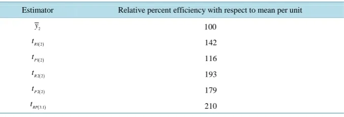
Table 1shows the percent relative efficiency of existing and proposed estimator with respect to mean per unit

estimator for two-phase sampling. It is observed that ratio and product estimators using one auxiliary attribute are more efficient than mean per unit in the two-phase sampling. Again, ratio and product estimator using multiple auxiliary attributes are more efficient than mean per unit and ratio and product estimator using one auxiliary attribute in the two-phase sampling. Finally, Ratio-cum-product estimator in the two-phase sampling for full in- formation case using multiple auxiliary attributes is the most efficient of the five estimators since it has the highest percent relative efficiency.

Table 2 shows percent relative efficiency of ratio-cum-product estimators with respect to mean per unit es-

timator in two-phase sampling. It is observed that the ratio-cum-product estimators are more efficient than mean per unit in the second phase sampling.

Finally,Table 3 compares the efficiency of full information case and partial case to no information case and full to partial information case. It is observed that the full information case and partial information case are more ef-ficient than no information case because they have higher Percent Relative Efficiency than no information case. In addition, the full information case is more efficient than the partial information case because it has a higher Per-cent Relative Efficiency than partial information case.

5. Conclusion

[image:11.595.143.482.110.225.2]

Table 1. Relative efficiency of existing and proposed estimator with respect to mean per unit estimator for two-phase sampling.

Estimator Relative percent efficiency with respect to mean per unit

2

y 100

( )

1 2

R

t ₁₄₂

( )

1 2

P

t ₁₁₆

( )

2 2

R

t ₁₉₃

( )

2 2

P

t ₁₇₉

( )3.1

RP

[image:11.595.141.487.258.348.2]

t ₂₁₀

Table 2. Relative efficiency of existing and proposed estimators with respect to mean per unit estimator for two-phase sampling.

Estimator Relative efficiency of existing and proposed estimators with respect to

mean per unit estimator for two-phase sampling

2

y 100

( )3.3

RP

t 135

( )3.2

RP

t 162

( )3.1

RP

t 211

Table 3. Comparisons of full, partial and no information cases for proposed ratio-cum-pro- duct estimator using multiple auxiliary variables.

Population _{full and partial to no information} Percent relative efficiency of Percent relative efficiency of full _{to partial in formation case}

Estimator tRP( )3.2 tRP( )3.1 tRP( )3.0 tRP( )3.1 tRP( )3.0

Relative percent

efficiency 100 130 168 100 135

mation case should be used but if all the auxiliary attributes are unknown, and ratio-cum-product estimator using multiple auxiliary attributes in no information case should be used to estimate finite population mean. This is clear from Table 3.

References

[1] Cochran, W.G. (1940) The Estimation of the Yields of the Cereal Experiments by Sampling for the Ratio of Grain to Total Produce. The Journal of Agricultural Science, 30, 262-275. http://dx.doi.org/10.1017/S0021859600048012 [2] Murthy, M.N. (1964) Product Method of Estimator. The Indian Journal of Statistics Series, 26, 69-74.

[3] Olkin, I. (1958) Multivariate Ratio Estimation for Finite Population. Biometrika, 45, 154-165. http://dx.doi.org/10.1093/biomet/45.1-2.154

[4] Raj, D. (1965) On a Method of Using Multi-Auxiliary Information in Sample Surveys. Journals of the American Sta- tistical Association, 60,154-165. http://dx.doi.org/10.1080/01621459.1965.10480789

[5] Singh, M.P. (1967) Multivariate Product Method of Estimation for Finite Population. Journal of the Indian Society of Agriculture Statistics, 31, 375-378.

[6] Singh, M.P. (1967) Multivariate Product Method of Estimation for Finite Population. Journal of the Indian Society of Agriculture Statistics, 31,375-378.

[7] Singh, H.P. and Tailor, R. (2003) Use of Known Correlation Coefficient in Estimating the Finite Population Mean.

Statistics in Translation, 6, 553-560.

[8] Naik, V.D. and Gupta, P.C. (1996) A Note on Estimation of Mean with Known Population of Auxiliary Character. Journal of the Indian Society of Agricultural Statistics, 48, 151-158.

[image:11.595.142.482.384.452.2]

159-163. http://dx.doi.org/10.1080/02522667.1991.10699058

[10] Rajesh, S., Pankaj, C., Nirmala, S. and Florentins, S. (2007) Ratio-Product Type Exponential Estimator for Estimating Finite Population Mean Using Information on Auxiliary Attributes. Renaissance High Press, USA.

[11] Jhajj, H.S., Sharma, M.K. and Grover, L.K. (2006) A Family of Estimator of Population Mean Using Information on Auxiliary Attributes. Pakistan Journal of Statistics, 22, 43-50.

[12] Neyman, J. (1938) Contribution to the Theory of Sampling Human Populations. Journal of the American Statistical Association, 33, 101-116. http://dx.doi.org/10.1080/01621459.1938.10503378

[13] Robson, D.S. (1952) Multiple Sampling of Attributes. Journal of the American Statistical Association, 47, 203-215. http://dx.doi.org/10.1080/01621459.1952.10501164

[14] Simiuddin, M. and Hanif, M. (2007) Estimation of Population Mean in Single and Two Phase Sampling with or with-out Additional Information. Pakistan Journal of Statistics, 23, 99-118.

[15] Hanif, M., Haq, I.U. and Shahbaz, M.Q. (2009) On a New Family of Estimator Using Multiple Auxiliary Attributes.

World Applied Science Journal, 11, 1419-1422.

[16] Haq, I.U. (2009) A Family of Estimators for Two-Phase Sampling Using Multi-Auxiliary Attributes. Ph.D. Thesis, Na- tional College of Business Administration & Economics, Lahore.