Numerical Study for Simulation the MHD Flow and Heat Transfer Due to a Stretching Sheet on Variable Thickness and Thermal Conductivity with Thermal Radiation

http://dx.doi.org/10.4236/am.2015.612180

Numerical Study for Simulation the MHD

Flow and Heat-Transfer Due to a Stretching

Sheet on Variable Thickness and Thermal

Conductivity with Thermal Radiation

Mohamed M. Khader

1,2

, Mohammed M. Babatin

1

, Ali Eid

3

, Ahmed M. Megahed

2 1_{Department of Mathematics and Statistics, College of Science, Al-Imam Mohammad Ibn Saud Islamic} University (IMSIU), Riyadh, Saudi Arabia

2_{Department of Mathematics, Faculty of Science, Benha University, Benha, Egypt}

3_{Department of Physics, College of Science, Al-Imam Mohammad Ibn Saud Islamic University (IMSIU), Riyadh,} Saudi Arabia

Received 6 October 2015; accepted 22 November 2015; published 25 November 2015 Copyright © 2015 by authors and Scientific Research Publishing Inc.

This work is licensed under the Creative Commons Attribution International License (CC BY).

http://creativecommons.org/licenses/by/4.0/

Abstract

The main aim of this article is to introduce the approximate solution for MHD flow of an electrically conducting Newtonian fluid over an impermeable stretching sheet with a power law surface velocity and variable thickness in the presence of thermal-radiation and internal heat generation/absorp- tion. The flow is caused by the non-linear stretching of a sheet. Thermal conductivity of the fluid is assumed to vary linearly with temperature. The obtaining PDEs are transformed into non-linear system of ODEs using suitable boundary conditions for various physical parameters. We use the Chebyshev spectral method to solve numerically the resulting system of ODEs. We present the effects of more parameters in the proposed model, such as the magnetic parameter, the wall thickness pa-rameter, the radiation papa-rameter, the thermal conductivity parameter and the Prandtl number on the flow and temperature profiles are presented, moreover, the local skin-friction and Nusselt numbers. A comparison of obtained numerical results is made with previously published results in some special cases, and excellent agreement is noted. The obtained numerical results confirm that the introduced technique is powerful mathematical tool and it can be implemented to a wide class of non-linear systems appearing in more branches in science and engineering.

Keywords

1. Introduction

The previous investigations ([1]-[6]) did not study the effects of radiation on the flow and heat transfer. In man-ufacturing industries, the radiative heat transfer flow is very important for the design of reliable equipments, nuclear plants, gas turbines and various propulsion devices for aircraft, missiles, satellites and space vehicles. Also, the effect of thermal radiation on the forced and free convection flows is important in the context of space technology and processes involving high temperature. Historically in ([7]-[10]), the study on boundary layer flows over a stretching sheet with variable thickness is presented. From these considerations, we can see that the effects of the non-flatness on the stretching sheet problems considering a variable sheet thickness have not pre-sented. So, the main goal of this paper is to introduce the numerical simulation using Chebyshev spectral method ([11]-[16]) for the proposed model.

2. Formulation of the Model

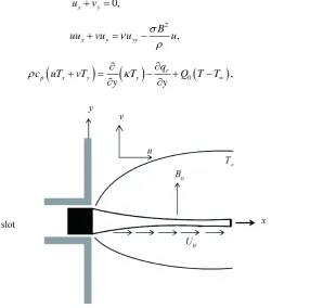
In this section, we will consider a steady, 2Dim boundary layer flow of an incompressible Newtonian fluid over a continuously impermeable stretching sheet. The origin is located at a slit, through which the sheet is drawn through the fluid medium (seeFigure 1). The velocity of the stretching surface is given by U_w=U₀

(

x b+

)

m, where U₀ is the reference velocity. We suppose that the sheet is not flat and defined as

(

)

1 2

m

y A x b

−

= + ,

where A is a very small constant so that the sheet is sufficiently thin and m is the velocity power index. We must note that the proposed model is satisfied only for m≠1, because for m=1, the model changes to a flat sheet. Likewise, the fluid properties are assumed to be constant except for thermal conductivity variations in the tem-perature. In this work, we will suppose that the variable magnetic field B x

( )

is applied normal to the sheet and that the induced magnetic field is neglected, which is justified for MHD flow at small magnetic Reynolds number.

In case of approximations for the usual boundary layer of the Newtonian fluid, we can write, the steady 2D im boundary-layer equations taking into account the thermal radiation effect in the energy equation in the following form:

0,

x y

u +v = (1) 2

,

x y yy

B uu vu νu σ u

ρ

+ = − (2)

(

)

( )

0

(

)

,

r

p x y y

q

c uT vT T Q T T

y y

ρ + = ∂ κ −∂ + − _∞

[image:2.595.189.476.421.705.2]

∂ ∂ (3)

where u and v are the velocity components in the x and y directions, respectively.

ρ

and

κ

are the fluid den-sity and the thermal conductivity, respectively. T is the temperature of the fluid, ν is the fluid kinematic vis-cosity, B is the strength of the applied magnetic field, c_p is the specific heat at constant pressure, σ is the electrical conductivity of the fluid, Q₀ is the heat generation/absorption coefficient and q_r is the radiative heat flux.

The radiative heat flux q_r is employed according to Rosseland approximation [17] such that

* 4 * 4 , 3 r T q y k σ ∂ = −

∂ (4)

where σ*=5.6697 10× −8W m⋅ −2⋅K−4 is the Stefan-Boltzmann constant and k* is the mean absorption coef-ficient. Following Raptis [18], we assume that the temperature differences within the flow are sufficiently small such that 4

T may be expressed as a linear function of the temperature. Expanding 4

T in a Taylor series about

T∞ and neglecting higher-order terms, we have

4 3 4

4 3 .

T ≅ T T∞ − T∞ (5) The physical and mathematical advantage of the Rosseland formula (4) consists of the fact that it can be com-bined with Fourier’s second law of conduction to an effective conduction-radiation flux q_eff in the form

* 3 * 16 , 3 eff eff

T T T

q

y y

k

σ

κ ∞ κ

  ∂ ∂

= −_ + _ = −

∂ ∂

  (6)

where * 3 * 16 3 eff T k σ

κ _{= +}κ ∞ _{is the effective thermal conductivity. So, the steady energy balance equation include-}

ing the net contribution of the radiation emitted from the hot wall and absorbed in the colder fluid, takes the form

(

)

0 .

p eff

T T T

c u v Q T T

x y y y

ρ _ ∂ + ∂ _= ∂ _κ ∂ _+ − _∞

∂ ∂ ∂ ∂

    (7)

To obtain similarity solutions, it is assumed that the magnetic field B x

( )

is of the form

( )

(

)

1

2

0 ,

m

B x B x b

−

= + (8)

where B₀ is the constant magnetic field. The boundary conditions can be written as

(

)

1

(

)

(

)

1

(

)

1

2 2 2

0

, , , 0, , ,

m m m

m

w

u x A x b U x b v x A x b T x A x b T

− − −

 ₊ _{= +}  ₊ ₌  ₊ ₌

     

      (9)

(

,

)

0,

(

,

)

.

u x ∞ = T x ∞ =T∞ (10) The mathematical analysis of the problem is simplified by introducing the following dimensionless coor- dinates

(

)

_{( )}

₍

₎

_{( )}

( )

1 1 0 0 1 2 , , , 2 1 , m m w x b m

y U x y U x b f

m T T

T T

η ψ ν η

ν θ η − + ∞ ∞  ₊  +  _{ }   = _{  } = _{ } + +  _{ }    −  =  ₋    (11)

where

η

is the similarity variable, ψ

( )

x y, is the stream function which is defined in the classical form as

u= ∂ψ ∂y and v= −∂ψ ∂x and θ η

( )

is the dimensionless temperature.

In this study, the equation for the dimensionless thermal conductivity

κ

is generalized for the temperature dependence as follows ([19][20]):

(

1

)

,

κ κ= ∞ +εθ (12)

Upon using these variables, the boundary layer governing Equations (1)-(3) can be written in a non-dimensional as follows 2 2 0, 1 m

f ff f Mf

m

′′′+ ′′− ′ − ′=

+ (13)

(

)

(

2

)

1

1 0,

R

f

Pr εθ θ εθ θ γθ

+

  _{+ ′′+ ′ + ′+ =}

 

  (14)

where

(

)

2 0 2 1 B M U m σ ρ =

+ is the magnetic parameter,

p

c

Pr µ

κ∞

= is the Prandtl number,

* 3 * 16 3 T R k σ

κ∞∞

= is the

rad-iation parameter and

(

)

(

)

1 0 0 2 1 m p

Q x b m c U

γ

ρ

− + =

+ is the heat generation parameter (>0) or the absorption parameter (<0).

Also, the boundary conditions transformed to the following form

( )

1

( )

( )

, 1, 1,

1

m

f f

m

α =α_ − _ ′ α = θ α = +

  (15)

( )

0,

( )

0,

f′ ∞ = θ ∞ = (16)

where 0

(

1

)

2 U m A α ν +

= is a parameter related to the thickness of the wall and 0

(

1

)

2 U m A η α ν +

= = indi-

cates the plate surface. We can write the Equations (13)-(14) in a simple form and to facilitate the computation, if we take into the account the transformation F

( )

ζ =F

(

η α−

)

= f

( )

η and Θ

( )

ζ = Θ

(

η α−

)

=θ η

( )

. So, the similarity equation and the associated boundary conditions become

2 2

0, 1

m

F FF F MF

m

′′′+ ′′− ′ − ′=

+ (17)

(

)

(

2

)

1

1 0,

R

F

Pr ε ε γ

+

  _{+ Θ Θ + Θ + Θ + Θ =′′ ′ ′}

 

  (18)

( )

1

( )

( )

0 , 0 1, 0 1,

1

m

F F

m

α −  ′

= _{ } = Θ =

+

  (19)

( )

0,

( )

0.

F′ ∞ = Θ ∞ = (20) The physical quantities of primary interest are the local skin-friction coefficient Cf and the local Nusselt number Nu which are defined as

( )

( )

1 1

2 2

1 1

2 0 , 0 ,

2 x 2 x

m m

Cf Re F Nu Re

−

+ _′′ + _′

= − = − Θ (21)

where w

x

U X Re

ν

= is the local Reynolds number and X = +x b.

3. Application of Chebyshev Spectral Method

In this section, we implement Chebyshev spectral method to solve the resulting system of non-linear ODEs of the form (17)-(18) with boundary conditions (19)-(20). To achieve this aim, and since the Gauss-Lobatto nodes

inside

[

−1,1

]

, we will use the transformation

(

1

)

2 x

η

3 2

2

2 2 2 2

0, 1

m

F FF F M F

m

η∞ η∞ η∞

  _′′′+   _{′′− ′} ₋   _′=

    _{ +} _  

      (22)

(

)

(

)

2

2

1 2 2

1 0,

R

F

Pr η_∞ ε ε η_∞ γ

   

+

  _{+ Θ Θ + Θ′′ ′ + Θ + Θ =′}

   

 

     (23)

also the boundary conditions will transform to the following form

( )

1

( )

( )

( )

( )

1 , 1 , 1 0, 1 1, 1 0,

1 2

m

F F F

m

η

α −  _′ ∞ _′

− = _{ } − = = Θ − = Θ =

+

  (24)

where F x

( )

and Θ

( )

x are unknown functions from Cm

[

−1,1

]

. Where the derivative in (22)-(23) will be w.r.t. the new variable x. The proposed technique is accomplished by starting with a Chebyshev approximation for the highest order derivatives, F( )3 and Θ( )2 and generating approximations to the lower order derivatives

( )

, 0,1, 2

i

F i= and Θ( )i,i=0,1 as follows: Setting F( )3

( ) ( )

x =

φ

x and Θ( )2

( ) ( )

x =

ξ

x , then by integration we obtain F( )2

( )

x , F( )1

( )

x , F x

( )

, Θ( )1

( )

x and Θ

( )

x as follows:

( )

_{( )}

_{( )}

( )

_{( )}

_{( )}

₍

₎

( )

( )

(

)

(

)

2 0 1 1 0 1 1 1 2

0 1 2

1 1 1

d ,

d d 1 ,

1 1

d d d .

2! 1!

x

x x

x x x

F x x x c

F x x x x x c c

x x

F x x x x x c c c

φ φ φ − − − − − − = + = + + + + + = + + +

∫

∫ ∫

∫ ∫ ∫

(25) ( )

_{( )}

_{( )}

( )

( )

(

)

1 0 1 0 1 1 1 ,

d d 1 .

x

x x

x x d

x x x x x d d

ξ

ξ −

− −

Θ = +

Θ = + + +

∫

∫ ∫

(26)

Also using the boundary conditions (24), the constants of integration c dk, k,k=0,1, 2, can be written as follows

( )

1

0 _{1 1} 1 2

1 1

d d , , ,

4 2 2 1

x m

c x x x c c

m

η_{∞ φ} η_{∞ α}

− − −   = − − = _{=  } +  

∫ ∫

( )

1

0 _{1 1} 1

1 1

d d , 1.

2 2

x

d = − −

∫ ∫

_{− −}

ξ

x x x d =

Now, the approximations to the Equations (25) and (26) will take the following forms

( ) ( )

( )

_{( )}

(

)

(

)

(

)

1 1 1 2 2 2

0 0 0

1 1 1

0 0

2

3 2 1 2 2 2 2

2 2

, , ,

, , 0 1 , and

0.25 1 , 0.5 1 , 0.5 ,

0.5 1

n n n

f f f f f f

i ij j i i ij j i i ij j i

j j j

n n

i ij j i i ij j i

j j

f f f

ij ij i nj ij ij i nj ij ij nj

ij ij i nj

f c f c f c

d d i n

b x b b x b b b

b x b

θ θ θ θ

θ

φ φ φ

θ ξ θ ξ

= = = = = = + = + = + = + = + ∀ = = − + = − + = − = − +

∑

∑

∑

∑

∑

        

(

)

(

)

(

)

(

)

1 2

2 _{1 2}

1

1

, ,

2 1

1 1 , 1 , ,

2 8 1 2 4 4

1 1

1 1, ,

2 2

ij ij nj

f f f

i i i i i i

i i i

b b

m

c x x c x c

m

d x d

θ

θ θ

η_∞ η_{∞ α} η_∞ η_∞ η_∞

= − −   = + − + + _{ } = − + = − +   = − + + = −

 (27)

where

(

)

(

)

2

2 3

, ,

2!

i j

ij i j ij ij ij

x x

linear equations in the highest derivative as follows:

( )

( )

( ) 2 2 ( )

2 2 1 1

0,

2 1 2

i i i i i

m

f f f M f

m

η η

φ ₊ ∞ ₋ ₋  ∞ ₌

 

 _{ + }  

    (28)

(

)

( )

( ) 2 ( ) 2

1 1

1

1 0.

2 2

i i i i i i

R

f Pr

η η

εθ ξ ε θ ∞ θ γ ∞ θ

+    

 _{ + +} _{+ + =}

 _{ }    

      (29)

These equations are non-linear system of 2n + 2 algebraic equations in 2n + 2 unknowns φ_i and ξ =i,i 0 1

( )

n. After solving this system using Newton’s iteration method and substitution φ_i and ξ_i in Equation (27), we can obtain the numerical solution of the system of Equations (17)-(18).

4. Results and Discussion

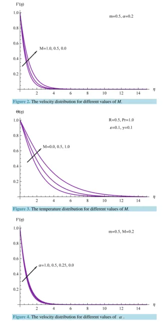
In Table 1 and Table 2, we presented the numerical solution using the Chebyshev spectral method with n=10. These results show excellent agreement with the existing solutions in the literature [10] and show that the pro-posed method suits for MHD boundary layer flow problems. Also, in this section we provided the behavior of parameters involved in the expressions of heat transfer characteristics for the stretching sheet. The numerical solutions of this problem are performed and illustrated graphically in Figures 2-11. Effects of the magnetic pa-rameter M on velocity and temperature profiles are shown in Figure 2 and Figure 3, respectively. It is observed that the velocity decreases for increasing values of M. Furthermore, the momentum boundary layer thickness decreases as M increases. This is due to the fact that as M increases, the boundary layer flow acquires more magnetization that leads to the variation in Lorentz force which opposes the flow. FromFigure 3, we can see that the fluid temperature increases when the magnetic number is increase, because Lorentz force which pro-duces from the presence of transverse magnetic field. When this force increases, the fluid exhibits a resistance to this force by increasing the friction between its layers. The increasing in the temperature caused by this resistance.

In Figure 4, Figure 5, we presented the obtained numerical results to show the effects of wall thickness pa-rameter on the fluid flow and the temperature distribution. From Figure 4, we can see that the velocity at any point near to the plate decreases as the wall thickness parameter increases. Also from these figures, we can note that the thickness of the boundary layer becomes thinner for a higher value of α and becomes thicker for a smaller value of α.

Figure 5 displays that the wall thickness parameter decreased the thickness of the thermal boundary layer and enhanced the rate of heat transfer. Physically, increasing the value of α will decrease the flow velocity be-cause under the variable wall thickness, not all the pulling force of the stretching sheet can be transmitted to the fluid causing a decrease for both friction between the fluid layers and temperature distribution for the fluid. Likewise, for a higher value of α, the thermal boundary layer becomes thinner compared with the smaller val-ue of the same parameter.

Table 1. The approximate values of −F′′

( )

0 , obtained by Chebyshev spectral technique with n=10 for α =0.5,

0

M = and [10].

m 10.00 9.00 7.00 5.00 3.00 1.00 0.50 0.00 −1/3 −0.50

( )0

F′′

− 1.0603 1.0589 1.0550 1.0486 1.0359 1.0000 0.9799 0.9576 1.0000 1.1667

Present work 1.0603 1.0588 1.0551 1.0486 1.0358 1.0000 0.9798 0.9577 1.0000 1.1666

Table 2. The approximate values of −F′′

( )

0 , obtained by Chebyshev spectral technique with n=10 for α =0.25,

0

M = and [10].

m 10.00 9.00 7.00 5.00 3.00 1.00 0.50 0.00 −1/3 −0.50

( )0

F′′

− 1.1433 1.1404 1.1323 1.1186 1.0905 1.0000 0.9338 0.78439 0.5000 0.0833

[image:7.595.145.475.81.728.2]

Figure 2.The velocity distribution for different values of M.

[image:7.595.171.457.507.719.2]

Figure 3.The temperature distribution for different values of M.

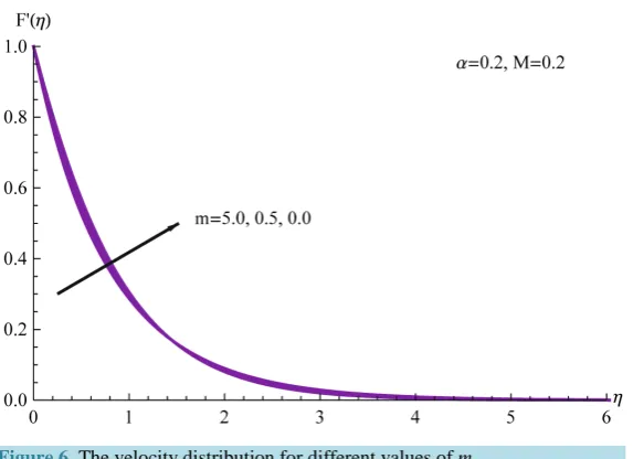
FromFigure 6, we can ensure that the velocity increases with a decrease in the values of the velocity power index m along the sheet and the reverse is true away from it. This implies that the momentum boundary thick-ness becomes thicker as m increases.

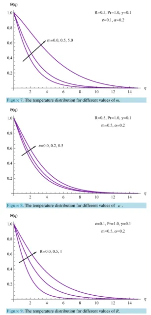
The influence of the velocity power index parameter m on the temperature profiles is displayed in Figure 7. From this figure, we can see that increasing the value of m produces an increase in the temperature profiles. It further shows that the larger the value of m, the higher the magnitude of the thermal boundary thickness will be.

From Figure 8, we can reveal that the temperature profile as well as the thickness of the thermal boundary layer increase when ε increases. Where in this figure, we have changed the thermal conductivity parameter ε with fixed the values of all other parameters.

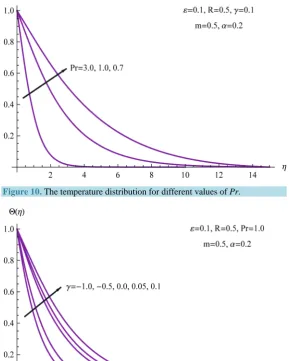
[image:8.595.166.467.291.723.2]

In Figure 9, we presented the effects of R on the temperature profiles with fixed the values of all other para-meters. From this figure, we noted that the temperature field and the thermal boundary layer thickness increase with the increase in R. Also, from Figure 10, we can observe that an increase in the Prandtl number results in decreases the heat transfer profiles. The reason is that increasing values of Prandtl number equivalent for de-creasing the thermal conductivities and therefore heat is able to diffuse away from the heated sheet more rapidly. Hence in the case of increasing Prandtl number, the boundary layer is thinner and the heat transfer is reduced.

[image:8.595.173.458.300.496.2]

Figure 11 illustrates the affect on the profiles of temperature distribution with different values of the parame-ter

γ

where we fixed all values of the other parameters. This figure indicates that the temperature distribution

Figure 5. The temperature distribution for different values of α.

[image:8.595.172.459.510.718.2]

[image:9.595.157.465.81.721.2] [image:9.595.171.455.86.288.2]

Figure 7.The temperature distribution for different values of m.

Figure 8. The temperature distribution for different values of ε .

[image:9.595.172.456.513.708.2]

[image:10.595.168.458.95.457.2] [image:10.595.171.456.301.511.2]

Figure 10. The temperature distribution for different values of Pr.

Figure 11. The temperature distribution for different values of γ .

increase when the internal heat generation parameter γ >0 becomes stronger whereas the internal heat absorp-tion parameter γ <0 have the opposite effect. Also, we can note that the highest temperature distribution for fluid in boundary layer was obtained with the greatest heat generation parameter γ >0. Likewise, it is shown that the effect of γ <0 causes a drop in the temperature distribution as the heat following from the sheet is ab-sorbed.

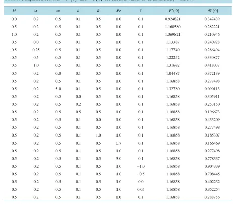
Table 3 shows the influence of the magnetic parameter M, wall thickness parameter α, the velocity power index parameter m, the radiation parameter R, the Prandtl number Pr, the heat generation/absorption parameter

[image:11.595.78.541.95.500.2]

Table 3.Comparison between −F′′

( )

0 and −Θ

( )

0 for different values of M, , , , ,α mε Rγ and Pr.

M α m ε R Pr γ −F′′( )0 −Θ′( )0

0.0 0.2 0.5 0.1 0.5 1.0 0.1 0.924821 0.347439

0.5 0.2 0.5 0.1 0.5 1.0 0.1 1.168580 0.282221

1.0 0.2 0.5 0.1 0.5 1.0 0.1 1.369821 0.210946

0.5 0.0 0.5 0.1 0.5 1.0 0.1 1.13387 0.240928

0.5 0.25 0.5 0.1 0.5 1.0 0.1 1.17740 0.286494

0.5 0.5 0.5 0.1 0.5 1.0 0.1 1.22242 0.330877

0.5 1.0 0.5 0.1 0.5 1.0 0.1 1.31682 0.418037

0.5 0.2 0.0 0.1 0.5 1.0 0.1 1.04487 0.372139

0.5 0.2 0.5 0.1 0.5 1.0 0.1 1.16858 0.277498

0.5 0.2 5.0 0.1 0.5 1.0 0.1 1.32780 0.090113

0.5 0.2 0.5 0.0 0.5 1.0 0.1 1.16858 0.305911

0.5 0.2 0.5 0.2 0.5 1.0 0.1 1.16858 0.253150

0.5 0.2 0.5 0.5 0.5 1.0 0.1 1.16858 0.196673

0.5 0.2 0.5 0.1 0.0 1.0 0.1 1.16858 0.433209

0.5 0.2 0.5 0.1 0.5 1.0 0.1 1.16858 0.277498

0.5 0.2 0.5 0.1 1.0 1.0 0.1 1.16858 0.185307

0.5 0.2 0.5 0.1 0.5 0.7 0.1 1.16858 0.166469

0.5 0.2 0.5 0.1 0.5 1.0 0.1 1.16858 0.277498

0.5 0.2 0.5 0.1 0.5 3.0 0.1 1.16858 0.778337

0.5 0.2 0.5 0.1 0.5 1.0 −1.0 1.16858 0.904339

0.5 0.2 0.5 0.1 0.5 1.0 −0.5 1.16858 0.708445

0.5 0.2 0.5 0.1 0.5 1.0 0.0 1.16858 0.402232

0.5 0.2 0.5 0.1 0.5 1.0 0.05 1.16858 0.352254

0.5 0.2 0.5 0.1 0.5 1.0 0.1 1.16858 0.288756

5. Conclusion

In this work, we implemented the Chebyshev spectral method to solve the non-linear system of ODEs of the proposed model. The fluid thermal conductivity is assumed to vary as a linear function of temperature. Asyste-matic study on the effects of the various parameters on flow and heat transfer characteristics is carried out. It has found that the effect of increasing values of the magnetic parameter, the velocity power index parameter, ther-mal conductivity parameter and the radiation parameter reduce the local Nusselt number. On the other hand, it is observed that the local Nusselt number increases as the Prandtl number and wall thickness parameter increases. Moreover, it is interesting to find that as the magnetic parameter, wall thickness parameter and the velocity power index parameter increases in magnitude, causes the fluid to slow down past the stretching sheet, the skin-friction coefficient increases in magnitude. A comparison with previously published work is given to en-sure that the obtained numerical results are in excellent agreement, and this confirms that the validity of the proposed method to solve the presented model. Finally, we can make the error is smaller by increasing the terms in the series (27). All computations in this paper are done using Mathematica 8.

Acknowledgements

References

[1] Crane, L.J. (1970) Flow past a Stretching Plate. Zeitschrift für Angewandte Mathematik und Physik, 21, 645-647.

http://dx.doi.org/10.1007/BF01587695

[2] Gupta, P.S. and Gupta, A.S. (1979) Heat and Mass Transfer on a Stretching Sheet with Suction or Blowing. Canadian Journal of Chemical Engineering, 55, 744-746. http://dx.doi.org/10.1002/cjce.5450550619

[3] Soundalgekar, V.M. and Ramana, T.V. (1980) Heat Transfer past a Continuous Moving Plate with Variable Tempera-ture. Warme-Und Stoffuber Tragung, 14, 91-93. http://dx.doi.org/10.1007/BF01806474

[4] Grubka, L.J. and Bobba, K.M. (1985) Heat Transfer Characteristics of a Continuous Stretching Surface with Variable Temperature. Journal of Heat Transfer, 107, 248-250. http://dx.doi.org/10.1115/1.3247387

[5] Chen, C.K. and Char, M. (1988) Heat Transfer on a Continuous Stretching Surface with Suction or Blowing. Journal of Mathematical Analysis and Applications, 35, 568-580. http://dx.doi.org/10.1016/0022-247X(88)90172-2

[6] Hayat, T., Abbas, Z. and Javed, T. (2008) Mixed Convection Flow of a Micropolar Fluid over a Non-Linearly Stret-ching Sheet. Physics Letters A, 372, 637-647. http://dx.doi.org/10.1016/j.physleta.2007.08.006

[7] Hossain, M.A., Alim, M.A. and Rees, D. (1999) The Effect of Radiation on Free Convection from a Porous Vertical Plate. International Journal of Heat and Mass Transfer, 42, 181-191.

http://dx.doi.org/10.1016/S0017-9310(98)00097-0

[8] Hossain, M.A., Khanfer, K. and Vafai, K. (2001) The Effect of Radiation on Free Convection Flow of Fluid with Va-riable Viscosity from a Porous Vertical Plate. International Journal of Thermal Sciences, 40, 115-124.

http://dx.doi.org/10.1016/S1290-0729(00)01200-X

[9] Bataller, R.C. (2008) Radiation Effects in the Blasius Flow. Applied Mathematics and Computation, 198, 333-338.

http://dx.doi.org/10.1016/j.amc.2007.08.037

[10] Fang, T., Zhang, J. and Zhong, Y. (2012) Boundary Layer Flow over a Stretching Sheet with Variable Thickness. Ap-plied Mathematics and Computation, 218, 7241-7252. http://dx.doi.org/10.1016/j.amc.2011.12.094

[11] Khader, M.M. (2015) Shifted Legendre Collocation Method for the Flow and Heat Transfer Due to a Stretching Sheet Embedded in a Porous Medium with Variable Thickness, Variable Thermal Conductivity and Thermal Radiation. Me-diterranean Journal of Mathematics, 1-18. http://dx.doi.org/10.1007/s00009-015-0594-3

[12] Khader, M.M. (2011) On the Numerical Solutions for the Fractional Diffusion Equation. Communications in Nonlinear Science and Numerical Simulation, 16, 2535-2542. http://dx.doi.org/10.1016/j.cnsns.2010.09.007

[13] Sweilam, N.H. and Khader, M.M. (2010) A Chebyshev Pseudo-Spectral Method for Solving Fractional Order Inte-gro-Differential Equations. ANZIAM Journal, 51, 464-475. http://dx.doi.org/10.1017/S1446181110000830

[14] Khader, M.M. and Megahed, A.M. (2013) Numerical Solution for the Effect of Fluid Properties Effect on the Flow and Heat Transfer in a Non-Newtonian Maxwell Fluid over an Unsteady Stretching Sheet with Internal Heat Generation.

Ukrainian Journal of Physics, 58, 353-361.

[15] Khader, M.M. and Megahed, A.M. (2014) Differential Transformation Method for Studying Flow and Heat Transfer Due to a Stretching Sheet Embedded in a Porous Medium with Variable Thickness, Variable Thermal Conductivity and Thermal Radiation. Applied Mathematics and Mechanics, 35, 1387-1400.

http://dx.doi.org/10.1007/s10483-014-1870-7

[16] Khader, M.M. and Megahed, A.M. (2014) Differential Transformation Method for the Flow and Heat Transfer Due to a Permeable Stretching Surface Embedded in a Porous Medium with a Second Order Slip and Viscous Dissipation.

Journal of Heat Transfer, 136, Article ID: 072602. http://dx.doi.org/10.1115/1.4027146

[17] Raptis, A. (1998) Flow of a Micropolar Fluid past a Continuously Moving Plate by the Presence of Radiation. Interna-tional Journal of Heat and Mass Transfer, 41, 2865-2866. http://dx.doi.org/10.1016/S0017-9310(98)00006-4

[18] Raptis, A. (1999) Radiation and Viscoelastic Flow. International Communications in Heat and Mass Transfer, 26, 889-895. http://dx.doi.org/10.1016/S0735-1933(99)00077-9

[19] Chiam, T.C. (1997) Magnetohydrodynamic Heat Transfer over a Non-Isothermal Stretching Sheet. Acta Mechanica,

122, 169-179. http://dx.doi.org/10.1007/BF01181997

[20] Mahmoud, M.A.A. and Megahed, A.M. (2009) MHD Flow and Heat Transfer in a Non-Newtonian Liquid Film over an Unsteady Stretching Sheet with Variable Fluid Properties. Canadian Journal of Physics, 87, 1065-1071.

http://dx.doi.org/10.1007/BF01181997