Brain Tumor Segmentation and Stage Detection in
Brain MR Images using K AMS EM Algorithm
Purnita Majumder
Research Scholar
Government College of Engineering Aurangabad, India
V. P. Kshirsagar
Head of the Department Government College of Engineering
Aurangabad, India
ABSTRACT
Image segmentation is often considered as a preliminary step in medical image analysis for computer aided diagnosis and therapy. Still it is tough to justify the accuracy of various segmentation algorithms, regardless the nature of the treated image. The abnormal growth of tissues reproducing themselves in any of the part body is called as tumor. There exist a various different types of tumor having different kind of Characteristics and treatment accordingly. As a result of imprecise detection of tumor a large number of people having brain tumors die every year. Due to the complex nature of medical image, analysis work of those is a challenging task. For early detection of abnormal behavior in human organs and tissues Magnetic resonance imaging (MRI) is an important diagnostic imaging technique which uses a combination of radio frequencies, large magnet and a computer to generate detailed images of organs and structures within the body. MR images are examined visually for detection of brain tumor producing less accuracy while detecting the stage & size of tumor.In this paper we propose the combination of K MEANS, AMS and EM algorithm for the detection of tumor stage in brain MR images and finding out the accuracy for those. In this method segmentation of tumor tissue is done with accuracy and reproducibility than manual segmentation with less analysis time. Also this accuracy is compared with the accuracy produced by the segmentation algorithms K MEAN and FCM combination. Then the tumor is extracted from the MR image and its exact shape, position and stage is determined.
General Terms
Segmentation, Clustering
Keywords
Brain tumor, Adaptive Mean-Shift (AMS), Expectation-Maximization (EM), K-means, Magnetic Resonance Imaging (MRI), Pre-processing, Support Vector Machine (SVM), Contrast Limited Adaptive Histogram Equalization( CLAHE).
1.
INTRODUCTION
This paper deals with automatic brain tumor segmentation and comparison of accuracy with previous existing system. There are various ways to view the anatomy of the Brain such as MRI scan or CT scan. In CT the effective radiation dose ranges from 2 to 10 mSv. While an average person receives the same from background radiation in 3 to 5 years. For pregnant women or children CT is not recommended usually. The MRI scan is more comfortable than CT scan for diagnosis. In this paper we consider the MRI scanned image for the whole process. Among
different types of algorithm for brain tumor detection, in this paper we used two algorithms for segmentation which gives the accurate result for tumor segmentation. More than 120 types of brain and central nervous system (CNS) tumors are existing. Almost all medical institutions use the World Health Organization (WHO) identification system to classify brain tumors. According to WHO brain tumors are classified by cell origin and the behavior of the cells, from the least aggressive (benign) to the most aggressive (malignant). Brain tumor normally affects CSF (Cerebral Spinal Fluid). It is the cause of strokes in the human body. So thepatients get the treatment for the strokes instead of the treatment for tumors. That’s why accurate detection of the tumor is important phase of the treatment. The lifespan of a brain tumor affected person can be increased if it is detected at current stage. It will help to maximize the lifetime by 1 to 2 years. We use MATLAB as the developing platform for the detection of tumor. We are providing systems that detect the tumor, its shape and the stage of a particular type of tumor. Then we will find out the accuracy of the proposed system for different MR images and then we will compare that with the previous existing system [1].
2.
PROPOSED SYSTEM
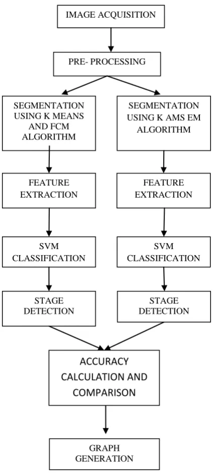
In this section, the main idea used in the proposed technique is described. The proposed system has mainly seven modules: preprocessing, segmentation, Feature extraction, Training and testing, Stage detection, Accuracy comparison, graph generation. In Pre processing Median filtering is performed on the MR image. Advanced K-mean, Adaptive mean shift and EM algorithms are used in segmentation work. Gray level Co-Occurance Matrix is used for feature extraction. And then SVM classifier is applied to detect whether the given image is Normal or Abnormal. Stage detection step is used to find out the stage of tumor which are marked as abnormal in previous step. Then we compare the accuracy of the proposed system with previous one. And Graph is generated to show the below 4 factors for the Proposed system and existing system.
Factors:
As shown the diagram below, the proposed system, is divided into the following 7 main phases:
[image:2.595.88.300.132.601.2]The flow for proposed system is shown in Figure 1.
Fig 1: Flow Diagram for Proposed System
2.1
PRE- PROCESSING
2.1.1
Image De-noising Using Adaptive
Median Filtering
In pre processing step the image is converted according to the need of the noise removal. Filtering of noise and other artifacts are performed on the image. Median filtering is used to reduce the salt-and-pepper or impulsive noise. Noise arrival possibilities in modern MRI scan are very less but due to the thermal effect it may appear. The main aim of this paper is tumor detection, tumor stage detection and comparison of accuracy with previous techniques. But for the better result, it needs the process of noise removal.
For this purpose Adaptive Median Filtering is proposed. Spatial processing is performed by the Adaptive Median Filter to find out those pixels in an image which have been affected by impulse noise. The AMF classifies pixels as noise by comparing each image pixel to its neighbor pixels. The size of the neighborhood and the threshold for the comparison is adjustable. Impulse noise is labeled as a pixel which is different from its majority of neighbors, also being structurally unaligned with the pixels similar to it. The median pixel value of those pixels in the neighborhood by which the noise labeling test have passed then replaces these noise pixels.
2.1.2
Image Enhancement Using Contrast
Limited Adaptive Histogram Equalization
After that, some image enhancement operations are performed to enhance the image by each layer. In this contrast enhancement techniques are applied using CLAHE Algorithm. This is an extension to the traditional Histogram Equalization technique. Contrast enhancement of the images is performed by transforming the values in the intensity image I. It operates on tiles (small data regions), rather than the entire image, unlike HISTEQ. Contrast Enhancement is performed on each tile, to match the histogram of the output region approximately with specified histogram. To eliminate artificially induced boundaries bilinear interpolation is used to combine the neighboring tiles. To avoid amplifying the noise which might be present in the image, the contrast, especially in homogeneous areas can be limited.Steps:
1. Obtain all the inputs: Image, Number of regions in row and column directions, Number of bins for the histograms used in building image transform function (dynamic range), Clip limit for contrast limiting (normalized from 0 to 1).
2. Pre-process the inputs: Determine real clip limit from the normalized value if necessary, pad the image before splitting it into regions.
3. Process each contextual region (tile) thus producing gray level mappings: Extract a single image region, make a histogram for this region using the specified number of bins, clip the histogram using clip limit, create a mapping (transformation function) for this region.
4. Interpolate gray level mappings in order to assemble final CLAHE image: Extract cluster of four neighboring mapping functions, process image region partly overlapping each of the mapping tiles, extract a single pixel, apply four mappings to that pixel, and interpolate between the results to obtain the output pixel; repeat over the entire image [2].
Algorithm:
1. Read the input image.
2. Convert input image into grayscale image if it is a color image.
3. Select the control parameter K1 and K2. 4. Calculate fmin and fmax. These are calculated as
follows:
fmin= min(min(f)) and PRE- PROCESSING
STAGE DETECTION
GRAPH GENERATION SEGMENTATION
USING K MEANS AND FCM ALGORITHM
IMAGE ACQUISITION
SEGMENTATION USING K AMS EM
ALGORITHM
FEATURE EXTRACTION
FEATURE EXTRACTION
SVM CLASSIFICATION
SVM CLASSIFICATION
STAGE DETECTION
ACCURACY
CALCULATION AND
COMPARISON
fmax= max(max(f)).
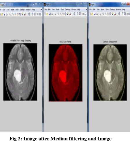
[image:3.595.80.305.134.378.2]5. Determine f=f-fmin and also Calculate f=f/fmax. 6. Convert the output image into uint8 format [3].
Fig 2: Image after Median filtering and Image enhancement
2.2
K AMS EM Algorithm
The proposed algorithm is the combination of K means, Adaptive mean shift clustering and Expectation Maximization algorithm. First we will describe the features of all the three algorithm. And then the proposed algorithm will be given.
2.2.1
K-MEANS Segmentation
One of the unsupervised learning algorithms for clusters is K-means. Grouping the pixels according to some characteristics is called clustering the image. Initially we have to define the number of clusters k in the k-means algorithm. Then randomly k-cluster center are chosen. The calculations of distance between each pixel to each cluster centers are done. That distance might be of simple Euclidean function. Using the distance formula all cluster centers are compared to Single pixel. Then the pixel is shifted to a particular cluster which is having the shortest distance among all. After that the centroid is re-estimated. Each pixel is compared to all centroids again and again. The process continues in this way until the center converges [1].
2.2.2
Segmentation Using Adaptive Mean Shift
Clustering
For imaging segmentation an automated scheme is proposed that is Adaptive Mean Shift Clustering. To classify brain voxels into three main tissue types as: white matter, gray matter, and Cerebrospinal fluid an AMS methodology is utilized. A high-dimensional feature space represents the image space that contains spatial features as well as multimodal intensity features. The clustering of the joint spatial-intensity feature space is done by AMS algorithm, within the feature space which extracts a representative set of high-density points, known as modes.
Tissue segmentation is achieved by an investigation phase of intensity-based mode clustering into the three categories of tissue. Adaptive mean-shift can deal well with non convex clusters by its nonparametric nature and yield convergence modes which are better options for intensity based classification as compared to the initial voxels.
2.2.3
Segmentation
Using
Expectation
Maximization
In expectation maximization (EM) algorithm an iterative method used to find out maximum likelihood measures of parameters in statistical models, where the model relies on unnoticed latent variables . The EM iteration takes turns between operating an expectation (E) step, which generates a function for the expectation of the log-likelihood calculated using the present estimate for the parameters, and the maximization (M) step, which evaluates parameters maximizing the anticipated log-likelihood that is found on the E step. To find out the distribution of the latent variables, these parameter-estimates are then used in the next E step.
Using the idea of above three algorithm the following algorithm is designed.
K AMS EM algorithm:
1. Digitize the image and get the pixel values.
2. Convert into double precision in order to increase the memory.
3. Calculate the normalized histogram.
The normalized histogram is used to calculate the clustering values for AMS EM algorithm. That decides the K value for the clustering.
4. Calculate the mean value for the normalized image.
5. Calculate the expectation pixels.
(Expectation pixels are called the unusual pixels which have unusual intensity. These pixels the calculated throughout the image and considered as expected pixel intensity).
6. Then calculate the maximization process, maximizing the expected pixel intensity and filtering the usual pixel intensity. This process is done by estimating the average of the expectation pixels and subtracting the average pixel intensity from the normalized pixels intensity.
7. Apply the thresholding value to the expectation maximization image in order to calculate the binary image.
8. Calculate the maxima from the thresholded image.
10. Build the m x n dimension for the given input image into the binary output.
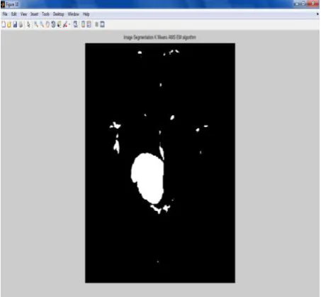
[image:4.595.79.306.123.332.2]Output:
Fig 3: Output of the K AMS EM algorithm
2.3
Feature Extraction Using Gray Level
Co-occurrence Matrix (Second Order
Feature Extraction)
2.3.1
Normalization of the Test Set
The images in the database are normalized before the co-occurrence matrices are calculated. To defeat the effects of monotonic transformations of the true image gray levels generated by difference of lightning, lens film and digitizers this idea is used. For all the images in the image database Normalization is carried out by setting standard and mean deviation to common values [3].
2.3.2
Grey
Level
Co-Occurrence
Matrix
(GLCM)
GLCM is a matrix that describes the frequency of one gray level appearing in a specified spatial linear relationship with another gray level within the area of investigation. The GLCM calculates how often a pixel with gray-level (grayscale intensity or Tone) value i occurs either horizontally, vertically, or diagonally to adjacent pixels with the value j [4] [5].
The Method:
Step 1: Obtain the co-occurrence matrices of each image. The gray levels of the image are reduced to 16. For 0 degree, 45 degree, 90 degree and 135 degree directions, and distances 1, 2, 3, 4 and 5, calculate the corresponding co-occurrence matrix. This produces 20 matrices of 16x16 integer elements per image.
Step 2: Obtain the values for the chosen descriptors. For each co-occurrence matrix, the value for the descriptor (or descriptors) is calculated. For each image, the resulting descriptor values are stored in a matrix where the rows represent the directions 0 degrees, 45 degrees, 90 degrees
and 135 degrees and the columns represent distances 1, 2, 3, 4 and 5.
Step 3: Generate image signatures. The image signatures are calculated from the descriptor matrix by averaging the values obtained with the different distances for each direction. Aiming at eliminating dependencies of image rotation, distances are calculated with different "rotations" on the elements of the signatures and the smaller one is adopted.
[image:4.595.329.554.235.448.2]Step 4: Compare the images through their signatures. The signatures of two images are compared and the distance between them is calculated, using the Euclidean distance function on the elements of the signature [6] [7].
Fig 4: GLCM Construction
After we create the GLCMs, you can derive several statistics from them using the different formulas.
In Our Project We have extracted features given below:
1. Autocorrelation-
* =
2. Amplitude (Intensity)-
3. Correlation-
4. Cluster Prominence-
5. Cluster shade-
6. Dissimilarity-
7. Energy-
8. Entropy-
9. Homogeneity-
10. Maximum Probability-
2.3.3
Splitting of the Images
Apparently some of the images may contain more than one texture. So, each of the original images is again divided into 9 sub images resulting in a database. For both split and original database retrieval results were produced. From each co occurrence matrix Entropy, Features energy, Inverse difference moment and Contrast are calculated and their values are recorded in the feature vector of the correlated image. Feature values within each feature class are normalized in the range [0, 1], to avoid features with greater values having more impact in the Euclidean distance (cost function) than features with smaller values. The similarity among images is calculated by summarizing Euclidean distances between corresponding features in their feature vectors. Those Images which are having feature vectors nearest to feature vector of the query image are given as best matches [6].
2.4
SVM Classifier
This Classification structures the data into different categories and investigates the numerical properties of image features. It has two steps of processing which are: training phase and testing phase. Characteristic properties of image features are collected and a unique definition of each classification category is created in Training phase. These features space partitions are used to categorize image features in testing phase.
A binary classifier depending on supervised learning that gives better execution than the other classifiers is known as SVM classifier. It classifies among two classes by creating a hyperplane in high-dimensional feature space that can be used in classification. Hyperplanes are represented by
w.x+b=0 (1)
W =weight vector and normal to hyperplane. B = threshold or bias.
Linear Separable Binary Classifier
Considering N training points, where each input has ‘A’ attributes and reside in one of two classes. Training data is of the form:
, i=1,2,….N;
ɛ
The main motive of using Support Vector Machine (SVM) is to align hyperplane in such a way as to be as far as possible from the closest members of both classes. Description of Training data is given by:
(w. + b) ≥ 1 for =+1 (2)
(w. + b) ≤ 1 for =-1 (3)
Equation (2) and (3) can also be written as:
(w. + b) -1 ≥ 0 (4)
Consider the points as that lie closest to the separating hyperplane, i.e. the Support Vectors; then the two planes; hyperplane 1 and hyper plane 2 lie on points which can be described as:
For Hyper plane 1, w. + b = +1 (5) For Hyper plane 2, w. + b = -1 (6)
Mathematics geometry analysis defined a distance from point P (m, n) to a line ax + by + c = 0
as
In the same way, the distance from a point x+ on HyperPlane1 to Optimal Hyperplane is given by d1 as
d1=
(7)
Similarly from a point X- on HyperPlane2 to Optimal Hyperplane is given by d2 as:
d2= (8)
By adding (7) and (8) we will get margin width
M=
(9)
Simple vector geometry in equation (9) shows that the margin is equal to 2/|w| and maximizing it subject to the constraint in (4) is equivalent to finding: min |w|
Subject to (w. + b) -1 ≥ 0 (10)
Minimizing ||w|| is equivalent to minimizing (the factor being used for mathematical convenience) and the use of this term makes it possible to perform Quadratic Programming (QP) optimization later on. We therefore need to find:
Applying above steps we can implement the Linear Separable Binary Classifier.
Whenever any new image comes for classification the trained data features and new image features are given to SVM classifier. In which the testing features are compared with the new features. If the result of comparing the both is highly matched then we put it to class 1, means the new image is Normal image. Else the features are placed into class 2, means the new image is infected image or abnormal image [8].
[image:6.595.331.548.152.506.2]OUTPUT:
Fig 5: Output of SVM classification
2.5
Stage Detection
Using the binarization method in the approximate reasoning step the area of the tumor is calculated. That means the image having two values either white or black (1 or 0). Here maximum image size is 256x256 jpeg image. We can represent a binary image as a summation of total number of black and white pixels [1].
Image, I=
Pixels = Height (H) X Width (W) = 256 X 256 f (l) = black pixel (digit 1)
f (0) = white pixel (digit 0)
No_of_white_pixel, P=
Where,
P = Total number of white pixels (height * width) 1 Pixel = 0.264 mm
The formula for area calculation is Size_of_tumor, S=
P= Number of white pixels; H=height, W=width;
ALGORITHM
The algorithmic steps involved for brain tumor shape detection is as follows-
Step 1: Start.
Step 2: Provide the MRI scan image in JPEG format as input.
Step 3: Check the input image format is as specified or not and go to step 4, display error message if not in specified format.
Step 4: Covert image into gray scale image if it is in RGB format else move to next step.
Step 5: Find the grayscale image edge.
Step 6: Calculate the total number of white points in the image.
Step 7: Using the formula calculate the size of the tumor. Step 8: Display the tumor size and stage.
Step 9: Stop the process.
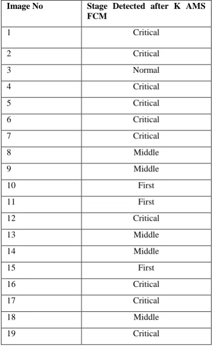
[image:6.595.80.292.212.296.2]The stage determination of tumor is based on the area of tumor. The proposed work uses techniques to calculate the tumor stage presented by J.selvakumar, A.Lakshmi, T.Arivoli in [9].
Table 1: Different Stages detected for Database Images Image No Stage Detected after K AMS
FCM
1 Critical
2 Critical
3 Normal
4 Critical
5 Critical
6 Critical
7 Critical
8 Middle
9 Middle
10 First
11 First
12 Critical
13 Middle
14 Middle
15 First
16 Critical
17 Critical
18 Middle
19 Critical
2.6
Accuracy Calculation and
Comparison
To measure the performance of the system for factors are calculated which in turn helps to calculate the accuracy of the proposed system and existing system.
True positive (TP): Tumor effected people correctly diagnosed as Abnormal.
False positive (FP): Normal people incorrectly identified as Abnormal means Tumor effected. True negative (TN): Normal people correctly
identified as healthy or Normal.
[image:7.595.325.551.52.539.2] False negative (FN): Tumor effected people incorrectly identified as healthy or Normal. Accuracy= (TP+FP) / (TP+TN+FP+FN) (12) Result generated for some images are shown in below table:
Table 2: Accuracy Comparison
Image No Accuracy For K FCM (%)
Accuracy For K AMS FCM(%)
1 84 93
2 76 90
3 65 76
4 56 76
5 80 88
6 37 68
7 54 78
8 82 94
9 84 94
10 90 96
11 84 95
12 53 81
13 93 97
14 82 95
15 85 95
16 82 93
17 87 90
18 82 95
19 91 93
2.7
Graph Generation
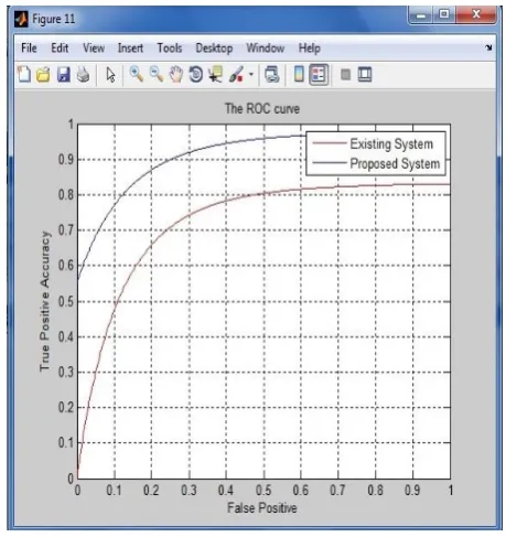
Each person going through the test either has or does not have the tumor. The result of the test can be positive or negative. The test outcome for each patient may or may not match the patient's actual status.
Using the factors TP, FP, TN, FN we have plotted the graph showing accuracy for the Proposed system and the existing system where values calculated for FP and TP are as below:
Table 3: Table for true positive and true negative values
False Positive (Reducing) True Positive (Increasing)
0.9962 0.9820
0.9962 0.9840
0.9962 0.9860
0.9961 0.9880
0.9961 0.9900
0.9961 0.9920
0.9960 0.9940
0.9960 0.9960
0.9960 0.9980
0.9959 1.0000
[image:7.595.71.299.239.607.2]OUTPUT:
Fig 6: ROC curve for True positive and False positive
3.
CONCLUSION
To remove any noise present in the input image Median filtering is applied and after that the CLAHE algorithm is performed on that. Input to the K AMS EM algorithm is the noise free image and tumor extraction operation is performed on the MRI image. Then features of the MR image are extracted and stored in feature matrix. These features are then compared with the trained features to classify whether the input image is Normal or Abnormal. Finally calculation of tumor stage detection is done using specific formulae. After that the experimental results are compared with other algorithms graphs will be generated. The result shows that the Proposed system is having more accuracy than the existing system. In future this system can be implemented with some other algorithm which will give more accuracy and save more time.
4.
ACKNOWLEDGMENT
[image:7.595.326.556.288.532.2]has been constant source of inspiration. She also thanks to Prof. M. B. Nagori, Professor, Computer Science & Engineering Depratment, Government College of Engineering, Aurangabad, for her valuable and firm suggestions.
5.
REFERENCES
[1] P.Majumder,V.Kshirsagar“Brain Tumor Segmentation and Stage Detection in Brain MR Images with 3D Assessment”, IJCA volume 84 2013. [2] Rajesh Garg, Bhawna Mittal, Sheetal Garg
“Histogram Equalization techniques for image enhancement” IJECT Vol. 2, Issue 1, March 2011. [3] Shyam Lal, Mahesh Chandra “Efficient Algorithm for
Contrast Enhancement of Natural Images”, The International Arab Journal of Information Technology, Vol. 11, No. 1, January 2014.
[4] M. M. Mokji, S.A.R. Abu Bakar “Gray Level Co-Occurrence Matrix Computation Based On Haar Wavelet”, Computer Graphics, Imaging and Visualisation (CGIV 2007).
[5] I. Felci Rajam and S. Valli “ A Survey on Content Based Image Retrieval”, Life Science Journal 2013; 10(2).
[6] Mari Partio, Bogdan Cramariuc, Moncef Gabbouj, and Ari Visa “ Rock Texture Retrival using Gray level Co-occurrence Matrix” Tampere University of Technology.
[7] Joaquim Cezar Felipe, Agma J. M. Traina, Caetano Traina Jr Retrieval by Content of Medical Images Using Texture for Tissue Identification. Institute of Superior Education COC.
[8] Daljit Singh, Kamaljeet Kaur “Classification of Abnormalities in Brain MRI images using GLCM,PCA and SVM” IJEAT ISSN: 2249 – 8958, Volume-1, Issue-6, August 2012.
[9] J.selvakumar, A.Lakshmi, T.Arivoli, “Brain tumor segmentation and its area calculation in brain MR images using K-mean clustering and fuzzy C-Mean algorithm”, 2012.
[10]Alan Wee-Chung Liew, Member, IEEE, and Hong Yan, Senior Member, IEEE, “An Adaptive Spatial
Fuzzy Clustering Algorithm for 3-D MR Image Segmentation”, in IEEE transactions on medical imaging, Vol. 22, No 9, Sept 2003.
[11]Jamal Ghasemi, Reza Ghaderi, Mohamad Reza Karami mollaei, Ali Hojjatoleslami “Separation of Brain Tissues in MRI based on Multi-Dimensional FCM and Spatial Information”, in FSKD-2011. [12]Linju Lu, Min Li, Xiaoying Zhang “An Improved MR
image segmentation method based on Fuzzy C-means Clustering”, in IJCSET 2013.
[13]Zexuan Ji, Yong Xia, Quansen Sun, Qiang Chen, Deshen Xia, David Dagan Feng “Fuzzy Local Gaussian Mixture Model for Brain MR Image Segmentation” in IEEE Transactions on Information Technology In Biomedicine, Vol. 16, No. 3, May 2012.
[14]Shally HR, Chitharanjan K,“Tumor volume calculation of brain from MRI slices”, 2013. [15]Mei Yeen Choong, Wei Yeang Kow, Yit Kwong
Chin, Lorita Angeline, Kenneth Tze Kin Teo, “Image Segmentation via Normalised Cuts and Clustering Algorithm”, in IEEE International Conference on Control System, Computing and Engineering, 2012. [16]Tse-Wei Chen , Yi-Ling Chen , Shao-Yi Chien, “Fast
Image Segmentation Based on K-Means Clustering with Histograms in HSV Color Space”, Journal of Scientific Research ISSN I452-2I6X Vol. 44 No.2, 2010.
[17]Anil Z Chitade, “Colour based imagesegmentation using k-means clustering”, in International Journal of Engineering Science and Technology, Vol. 2(10), 2010.
[18]T. Kanungo, D. M. Mount, N. Netanyahu, C. Piatko, R. Silverman, & A. Y.Wu, “An efficient k-means clustering algorithm:Analysis and implementation”, in Proc. IEEE Conf. Computer Vision and Pattern Recognition, 2002.