Calculating Dynamic Time Quantum for Round Robin Process Scheduling Algorithm

(1)

Calculating Dynamic Time Quantum for Round Robin

Process Scheduling Algorithm

Aashna Bisht

Department of Computer Science, Jamia Hamdard

New Delhi, India

Mohd Abdul Ahad

New Delhi, India

Sielvie Sharma

New Delhi, India

ABSTRACT

Process scheduling using Round Robin Algorithm makes use of a fixed amount of time quantum that is assigned to each process to complete its execution. If the process is able to complete its execution within this time period, it is discarded from the ready queue otherwise it goes back to the rear of the ready queue and waits for its next turn. In this paper we have presented amelioration to the conventional round robin algorithm by evaluating the time quantum on the basis of the burst times of the various processes waiting in the ready queue. The allocation of dynamic time quantum to various processes will have a direct impact on various performance parameters like turnaround time, waiting time, response time and the number of context switches. Further we are increasing the time quantum for the processes which require a fractional more time to complete their execution than the allocated time quantum cycle(s).

Keywords

Context Switches, Scheduling, Turnaround time, Wait time.

1. INTRODUCTION

Process scheduling may be defined as the policies and mechanism to allocate CPU to various processes [11], [12]. The fundamental aim of the operating system is to discharge the task of process management and its performance can be construed in terms of how well it administers different jobs coming to the CPU for execution [11], [12], [14]. A good scheduling policy ensures that the most crucial job(s) gets the intended resource (CPU time)[11], [12], [13]. The effectiveness of a processor can be inspected using the following parameters [11], [12], [13], [14].

1.1 Turnaround Time

It is defined as the time taken by the processes since their commencement till they execute completely [11], [17].

1.2 Wait Time

It is defined as the time consumed by the processes waiting in ready queue till the CPU is allocated to them [11], [12].

1.3 Throughput

It is defined as the rate of execution of the total number of processes [11], [12], [17].

1.4 Context switches

It is defined as the swapping of CPU between the processes [11], [12], [14], 1[7].

CPU until the first reaction [11], [12].

Few common Scheduling Algorithms include First Come First Serve (FCFS), Shortest Job First (SJF) and Round Robin (RR) algorithms [11], [12], [13], [14], [15], [17]. FCFS algorithm gives the CPU to the job that arrives first at the CPU for execution. The job is not preempted until it completes its execution [11], [12], [13], [17]. Shortest Job First algorithm gives the CPU to the process with the minimal burst time first, here also the job is not preempted until it completes its execution [11],[12], [13], [17]. Round Robin algorithm is philosophically similar to the FCFS algorithm however in this algorithm every job is assigned a fixed time quantum to complete its execution [11] [12], [13], [15], [17].

2. PRELIMINARIES

(2)

time of the processes. The authors of [19] compared various proposals on improving the conventional round robin algorithm.

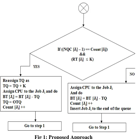
3. PROPOSED APPROACH

(3)

[image:3.595.56.293.69.311.2]

Fig 1: Proposed Approach

4. HYPOTHETICAL EXAMPLES

This section provides few hypothetical examples to show the working of the proposed approach as well as its comparison with the conventional round robin approach

[image:3.595.314.549.91.438.2]

4.1 Example 1

Table 1: Jobs Table with burst times for Conventional Round Robin Approach

Time Quantum (TQ) = 5

Job Name (Pi) Burst Time BT[Pi]

P1 19

P2 09

P3 23

P4 15

P5 16

Fig 2: Gantt chart using Conventional Round Robin Algorithm

4.1.1 Calculations using the Classical Round

Robin Algorithm:

Average Turnaround Time = (73+34+82+64+79)/5 = 66.4

Average Wait Time

= ((73-19) + (34-09) + (82-23) + (64-15) + (79-16) )/5

4.1.2 Calculation using the proposed Approach

Calculation of TQ: Max (BT) = 23 Min (BT) = 09

C =



([Max

(BT)

-

Min

(BT)]

/

2)



=



(23

-

09)

/

2 

=



14 / 2



= 7

Z =





(BT

[Pi])

/N)



= 16

As C < Z, Therefore TQ = 7 Calculation of K K=



_Z_/_TQ



=



16/7



= 2

Table 2: Jobs Table with burst times for Proposed Approach

Job Name

Pi

Burst Time BT[Pi]

Remaining Time RT[Pi]= BT[Pi]%TQ

Number of Cycles NQC[Pi] =



BT[P_i] / TQ



P1 19 5 3

P2 09 2 2

P3 23 2 4

P4 15 1 3

P5 16 2 3

Now as per the proposed approach we will modify the time quantum for those processes for which the remaining time is less than or equal to K. Other processes will be executed as per the conventional round robin algorithm with the original time quantum value. Here, those processes are P2, P3, P4, and P5 only. However, their time quantum will be increased only in the last but one CPU cycle. The figure given below depicts the Gantt chart using the proposed approach.

Fig 3: Gantt chart using Proposed Approach

Average Turnaround Time = (73+16+82+59+68) / 5 = 59.6

Average Wait Time

= ((73-19) + (16-09) + (82-23) + (59-15) + (68-16)) / 5 = (54+7+59+44+52) / 5

= 43.2

Number of Context switches = 10.

4.2 Example 2

[image:3.595.55.285.407.594.2]

(4)

[image:4.595.49.293.67.251.2]

4.2.1 Calculations as per Classical Round

Robin Algorithm:

Average Turnaround Time = (69+73+114+140+132) / 5 = 528/5

=105.6

Average Wait Time

= ((69-21) + (73-16) + (114-29) + (140-44) + (132-30))/5 = 388 / 5

= 77.6

4.2.2 Calculation as per proposed Approach

Max(BT) = 44 Min(BT) = 16

C =



_([Max

_(BT)

_-

_Min

_(BT)]

_/

₂₎



=



(44

-

16)

/

2 

=



28 / 2



= 14

Z =

_

((BT[Pi]) /N)

_

= 28

As C < Z,

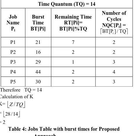
Therefore TQ = 14 Calculation of K K=



Z/TQ



=

_

₂₈_/₁₄

_

= 2

[image:4.595.318.549.81.315.2]

Average Turnaround Time = (79+30+94+140+124) / 5 = 467/ 5

= 93.4

Average Wait Time

= ((79-21) + (30-16) + (94-29) + (140-44) + (124-30) ) / 5 = (58+14+65+96+94) / 5

= 65.4

4.3 Example 3

Table 5: Jobs Table with burst times for Conventional Round Robin Algorithm

4.3.1 Calculations as per Classical Round

Robin Algorithm:

Average Turnaround Time = (79 +66+88+94+76 )/ 5 Time Quantum(TQ) = 12

Job Name (Pi) Burst Time BT[Pi]

P1 21

P2 16

P3 29

P4 44

P5 30

Job Name

Pi



BT[P_i] / TQ



P1 21 7 2

P2 16 2 2

P3 29 1 3

P4 44 2 4

P5 30 2 3

Time Quantum = 4

Process Name (Pi) Burst Time (BT[Pi])

P1 19

P2 14

P3 21

P4 26

(5)

= 403/5 = 80.6

Average Wait Time

= ( (79-19) + (66-14)+ (88-21) + (94-26)+ (76 -14) )/ 5 = (60 + 52+ 67+ 68+ 62)/ 5

= 309 / 5 = 61.8

Number of Context switches= 24.

4.3.2 Calculations as per proposed approach

Calculation of TQ: Max(BT) = 26 Min(BT) = 14

C =



_([Max_(BT)_-_Min_(BT)]_/₂₎



=



(26-14) / 2



=

_

12 / 2

_

= 6

Z =





(BT

[Pi])

/N)



= 18

As C < Z, Therefore TQ = 6 Calculation of K K=



Z

/

TQ



=



18/6



= 3

Average Turnaround Time = (71+44+ 80+94+64)/ 5 = 353/5

= (52 + 30 + 59 + 68+ 50)/ 5 = 259/5

= 51.8

5. RESULTS

[image:5.595.318.563.265.564.2]

In our proposal we are improving the conventional round robin algorithm in two ways, first by dynamically calculating the time quantum by sensing the burst times of the processes and secondly by further increasing the time quantum for the processes which need a fractional greater time than the allocated time quantum cycle(s) to complete their execution. The graphs and tables presented below provide a comparison between the proposed approach and the conventional round robin approach.

Table 7: Comparison table as per Example 1

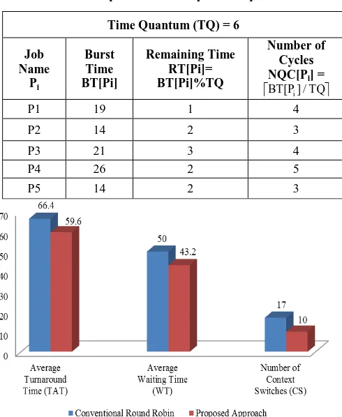
Fig 8: Comparison graph for Example 1 Comparison

Parameter Name

Conventional Round Robin

Proposed Approach

Improvement observed

Average Turnaround Time (TAT)

66.4 59.6 6.8 units of time saved

Average Waiting Time

(WT)

50 43.2 6.8 units of

time saved

Number of Context Switches(CS)

17 10

7 number of context switch

reduced

Job Name

Pi



BT[P_i] / TQ



P1 19 1 4

P2 14 2 3

P3 21 3 4

P4 26 2 5

(6)

[image:6.595.49.296.67.408.2]

Fig 9: Comparison graph for Example 2

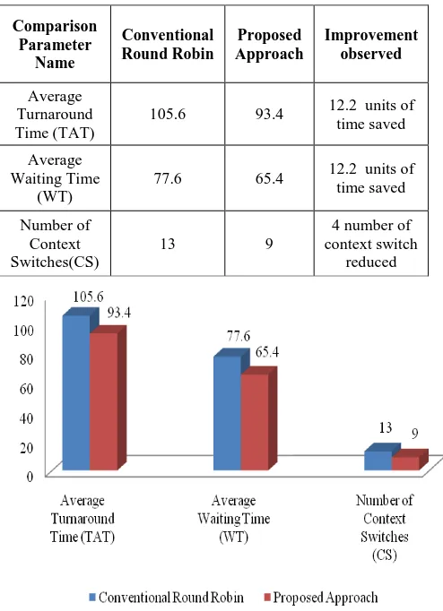
[image:6.595.319.555.73.226.2]

Table 9: Comparison table as per Example 3

Fig 10: Comparison graph for Example 3

6. CONCLUSIONS

From the above results it can be concluded that the proposed approach shows a clear edge over the conventional round robin algorithm. The approach can be further refined using the concept of fuzzy logic in order to calculate the dynamic time quantum.

7. REFERENCES

[1] Nayana Kundargi,Sheetal Bandekar,"CPU Scheduling Algorithm Using Time Quantum For Batch System",International Journal Of Latest Trends In Engeneering And Technology(IJLTET), special Issue- IDEAS 2013.

[2] Himanshi Arora,Deepanshu Arora,Bagish Goel,Parita Jain,"An Improved Scheduling Algorithm",International Journal of applied Information Systems(IJAIS), Foundation of Computer Science FCS, New York, USA, Volume 6– No. 6, December 2013, pp 7- 9.

[3] Sandeep Negi,"An Improved Round Robin Approach Using Dyanamic Time Quantum For Improving Average Waiting Time",International Of Computer Applications, Volume 69– No.14, May 2013, pp 12-16 .

[4] Rakesh Patel,Mrs.Mili. Patel," SJRR CPU Scheduling Algorithm "International journal of Engineering And Computer Science. Volume 2 Issue 12, Dec.2013 Pp: 3396-3399

[5] Adeeba Jamal,Aiman Jubair" A Varied Round Robin Approach Using Harmonic Mean Of The Remaining Burst Time Of Processes", Special Issue of International Journal of Computer Applications (0975 – 8887), 3rd International IT Summit Confluence 2012 - Pp 11- 17 .

[6] Mohd Abdul Ahad,"Modyfying Round Robin Algorithm For Process Scheduling Using Dynamic Quantum Precision", Special Issue Of International Journal of Computer Applications On Issues AND Challenges In Networking ,Intelligence And Computing Technologies, ICNICT 2012, November 2012, Pp 5-10.

[7] C.Yaashuwanth, Dr.R.Ramesh, A New Scheduling Algorithms for Real Time Tasks, (IJCSIS) International Journal of Computer Science and Information Security, Vol. 6, No.2, 2009, Pp: 61-66

Comparison Parameter

Name

(WT)

13 9

reduced

Comparison Parameter

Name

80.6 70.6 10 units of

time saved

(WT)

61.8 51.8 10 units of

time saved

24 12

(7)

[9] Lalit Kishor, Dinesh Goyal, Time Quantum Based Improved Scheduling Algorithm, Vol 3 , Issue International Journal of Advanced Research in Computer Science and Software Engineering. 4, April, 2013

[10] P. Surendra Varma, A Best possible time quantum for Improving Shortest Remaining Burst Round Robin (SRBRR) Algorithm, International Journal of Advanced Research in Computer Science and software Engineering, Volume 2, Issue 11, ISSN: 2277 128X , November 2012.

[11] Silberschatz, A. P.B. Galvin and G. Gagne (2012), Operating System Concepts, 8th edition, Wiley India

[12] Operating Systems Sibsankar Haldar 2009, Pearson.

[13] D.M. Dhamdhere operating Systems A Concept Based Approach, Second edition, Tata McGraw-Hill, 2006.

[14] Sanjaya Kumar Panda, Sourav Kumar Bhoi, An Effective Round Robin Algorithm using Min-Max Dispersion Measure, IJCSE, Vol. 4 No. 01, pp: 45-53 January 2012

[15] Prof. Bob Walker, Kathryn McKinley, Bradley Chen, Michael Rosenblum, Tom Anderson, John Ousterhout, Paul Farrell/Steve Chapin Operating system lectures

notes http://www.cs.kent.edu/~farrell/osf03/ oldnotes/L06.pdf

[16] Aashna Bisht, Mohd Abdul Ahad, Sielvie Sharma, “Enhanced Round Robin Algorithm for Process Scheduling using varying quantum precision” ,Proceedings of ICRIEST AICEEMCS, 29th December, 2013.pp 11-15.

[17] R. N. D. S. S Kiran, Polinati Vinod Babu, B. B. Murali Krishna,Optimizing CPU Scheduling for Real Time Applications Using Mean-Difference Round Robin (MDRR) Algorithm, ICT and Critical Infrastructure: Proceedings of the 48th Annual Convention of Computer Society of India- Vol I, Advances in Intelligent Systems and Computing Volume 248, 2014, pp 713-721. Springer International Publishing Switzerland, 2014.

[18] M.H. Zahedi, M. Ghazizadeh, M. Naghibzadeh, Fuzzy Round Robin CPU Scheduling (FRRCS) Algorithm, Advances in Computer and Information Sciences and Engineering, 2008, pp 348-353, Publisher Springer Netherlands,