Performance Evaluation of Face Recognition using
PCA and N-PCA
Ajay Kumar Bansal
Department of Electrical Engineering Poornima College of Engineering, Jaipur
Pankaj Chawla
Department of Electrical Engineering Poornima College of Engineering, Jaipur
ABSTRACT
Face recognition has become a valuable and routine forensic tool used by criminal investigators. It is an important area of computer vision research and has gained significant interest in recent years. Efforts in improving security, such as automatic surveillance and the use of biometrics in identification, are partly responsible for this increased interest. However, several challenges remain in improving the accuracy of face recognition under illumination changes, variations in pose, occlusions, and image resolution. This paper presents performance comparison of face recognition using Principal Component Analysis (PCA) and Normalized Principal Component Analysis (N-PCA). The experiments are carried out on the ORL, Indian face database and Georgia Tech face database which contain variability in expression, pose, and facial details. The results obtained for the two methods have been compared by varying the number of training images and it has been found that as the number of training images increases efficiency also increases. The result also shows that N-PCA gives better results than PCA.
General Terms
Face Recognition, Statistical Approach, Normalization.
Keywords
PCA, N-PCA, Feature Extraction and Euclidean distance.
1.
INTRODUCTION
As one of the few biometric methods that acquire the qualities of both low intrusiveness and high accuracy, Face Recognition Technology (FRT) has a range of applications in law enforcement and inspection, access control, information security, smart cards, among others [1-2]. For this reason, FRT has received significantly increased attention from both the academic and industrial communities during the past 20 years. Several authors have in recent times evaluated and surveyed the current FRTs from diverse aspects. For example, Smal et al. [3] and Valentin et al. [4] examined the neural network- based and the feature-based techniques, respectively, Yang et al. surveyed face detection techniques [5], Pantic and Rothkrantz [6] surveyed the automatic facial expression analysis, Daugman [2] pointed out several critical issues involved in an effective face recognition system, while the most latest and ample survey is possibly from that of Zhao et al [1], where many of the recent techniques are analyzed. The aim of face recognition is to identify or verify persons from motionless images using a stored database of faces.
Face recognition is basically the skill to set up a subject’s identity based on his facial description/features. Due to its significant role in a number of relevance fields, including visual inspection and de-duplication of government issued identity documents for instance passport and driver license, access control etc automatic face recognition has been broadly studied over the past three decades. Face recognition systems generally divided into two categories: identification or verification. In an identification set-up the similarity between a given face image and all the face images in a large database is computed; the top match is returned as the recognized identity of the subject. In a verification scenario, the similarity between two face images is measured and a determination of either match or non-match is made. Ideally, both of these categories are expected to work in a lights out mode that is the arrangement makes uniqueness decision without requiring any human interaction.
The skill to identify human faces is a demonstration of astonishing human intelligence. Over the last three decades researchers have been making attempts to study this outstanding visual perception of human beings in machine recognition of faces [7-8]. However, there are still substantial challenging problems such as intra class variations in 3D pose, make-up and illumination condition, facial appearance as well as occlusion and messed up background. To deal with these complications, various techniques have been projected which are discussed in further sections.
Different researchers for the face recognition system have proposed many linear and nonlinear statistical techniques. The PCA or Eigenfaces method [9], Independent Component Analysis (ICA) [10], and Linear Discriminant Analysis (LDA) [11], and PCA combined with LDA [12] are the most widely used linear statistical techniques reported by research community. Delac et al. [13] presented an autonomous, comparative study of three most accepted appearance-based face recognition methods (PCA, ICA, and LDA) in completely equal working conditions.
2.
FACE RECOGNITION SYSTEM
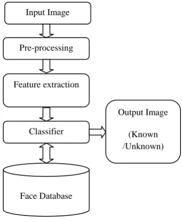
[image:2.595.98.279.203.424.2]A pattern recognition task performed exclusively on faces is termed as face recognition. It can be described as classifying a face either known or unknown, after matching it with stored known individuals as a database. It is also advantageous to have a system that has the capability of learning to identify unknown faces. The outline of typical face recognition system implemented specifically for N-PCA is given in Figure1. There are five main functional blocks, whose responsibilities are as below.
Fig 1: Block Diagram of face recognition system
A. The acquisition module
This is the entry point of the face recognition process. The user gives the face image as the input to face recognition system in this module.
B. The pre-processing module
In this module the images are normalized to improve the recognition of the system. The pre-processing steps implemented are as follows:
• Image size normalization
• Background removal
• Translation and rotational normalizations
• Illumination normalization
C. The feature extraction module
After the pre-processing the normalized face image is given as input to the feature extraction module to find the key features that will be used for classification. The module composes a feature vector that is well enough to represent the face image.
D. The classification module
With the help of a pattern classifier, the extracted features of face image are compared with the ones stored in the face
E. Face database
It is used to match the test image with the train images stored in a database. If the face is recognized as “unknown”, face images can then be added to the database for further comparisons.
3.
FACE RECOGNITION ALGORITHM
Face recognition systems are now replenishing the need for security to cope up with the current misdeeds. It is really influential with the market information that undoubtedly depicts the rising attractiveness of the face recognition system. In the present era, the threat of protecting the information or physical property is becoming more and more difficult and important. Now a day the crimes of computer hackings, credit card deception or security violation in a company or government building has noticed to be increased [14].
The face recognition system consists of two important steps, the feature extraction and the classification. Face recognition has a challenge to perform in real time. Raw face image may consume a long time to recognize since it suffers from a huge amount of pixels. One needs to reduce the amounts of pixels. This is called dimensionality reduction or feature extraction, to save time for the decision step. Feature extraction refers to transforming face space into a feature space. In the feature space, the face database is represented by a reduced number of features that retain most of the important information of the original faces [15]. The most popular method to achieve this target is through applying the Eigenfaces algorithm [9, 16]. The Eigenfaces algorithm is a classical statistical method using the linear Karhumen-Loeve transformation (KLT) also known as Principal component analysis. The PCA calculates the eigenvectors of the covariance matrix of the input face space. These eigenvectors define a new face space where the images are represented. In contrast to linear PCA, N-PCA has been developed.
3.1 Principal Component Analysis
Principal component analysis (PCA) is a statistical dimensionality reduction method, which produces the optimal linear least-square decomposition of a training set. Kirby and Sirovich [17] applied PCA for representing faces and Turk and Pentland [9] extended PCA for identifying faces. In applications such as image compression and face recognition a helpful statistical technique called PCA is utilized and is a widespread technique for determining patterns in data of large dimension. PCA commonly referred to as the use of Eigen faces [17].
The PCA approach is then applied to reduce the dimension of the data by means of data compression, and reveals the most effective low dimensional structure of facial patterns. The advantage of this reduction in dimensions is that it removes information that is not useful and specifically decomposes the structure of face into components which are uncorrelated and are known as Eigen faces [18]. Each image of face may be stored in a 1D array which is the representation of the weighted sum (feature vector) of the Eigen faces.In case of this approach a complete front view of face is needed; or else the output of recognition will not be accurate. The major benefit of this method is that it can trim down the data required to recognize the entity to 1/1000th of the data existing.
Input Image
Pre-processing
Feature extraction
Classifier
Face Database
Output Image
values. An image may also be considering the vector of dimension mn, so that a typical image of size 112x92 becomes a vector of dimension 10304. Let the training set of images {X1, X2, X3… XN}. The average face of the set is
defined by:
𝑋 = 𝑁1 𝑁𝑖=1𝑋𝑖 (1) Calculate the estimate covariance matrix to represent the scatter degree of all feature vectors related to the average vector. The covariance matrix C is defined by [2]:
𝐶 = 1
𝑁 𝑋 − 𝑋𝑖
𝑁
𝑖=1
𝑋 − 𝑋𝑖 T (2) The Eigenvectors and corresponding Eigen-values are computed by using
𝐶𝑉 = λV (𝑉 𝜖 𝑅𝑛 , 𝑉 ≠ 0 ) (3)
where V is the set of eigenvectors matrix C associated with its eigenvalue λ. Project all the training images of ith person to corresponding eigen-subspace:
𝑦𝑘𝑖 = 𝑤𝑇 𝑥𝑖 (𝑖 = 1,2,3 … … … … 𝑁) (4)
Where the yk are the projections of x and called the principal
components also known as eigenfaces. The dimensionality can be reduced by selecting the first N eigenvectors that have large variances and discarding the remaining ones that have small variance.
After feature extraction step next is the classification step which makes use of Euclidean Distance for comparing/matching of the test and trained images. In the testing phase each test image should be mean centred, now project the test image into the same eigenspace as defined during the training phase. This projected image is now compared with projected training image in eigenspace. Images are compared with similarity measures. The training image that is the closest to the test image will be matched and used to identify. Calculate relative Euclidean distance between the testing image and the reconstructed image of ith person, the minimum distance gives the best match.
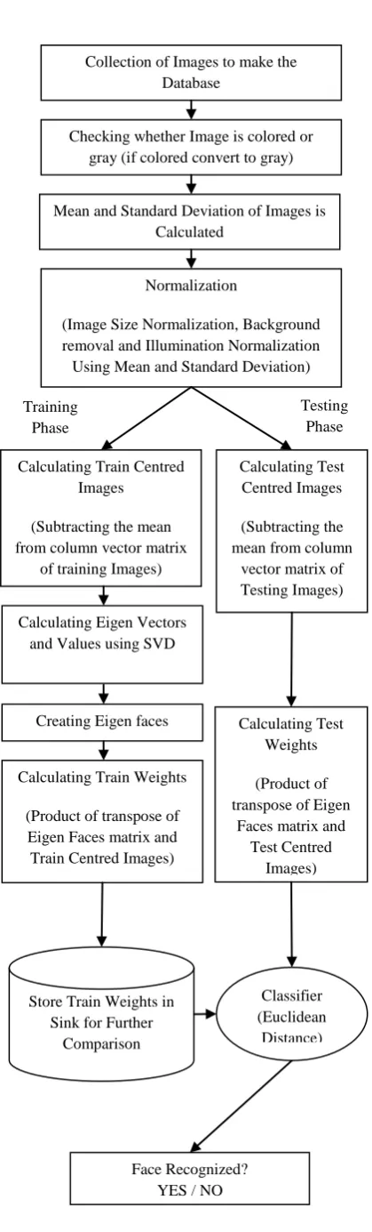
3.2 Normalized Principal Component
Analysis (N-PCA)
In contrast to linear PCA, N-PCA has been developed to give better results in terms of efficiency. N-PCA is an extension over linear PCA in which firstly normalization of images is done in order to remove the lightning variations and background effects and singular value decomposition (SVD) is used instead of eigen value decomposition (EVD), followed by the feature extraction steps of linear PCA and lastly in classification steps weights are calculated for matching purpose.
The Normalized PCA is developed by taking into account the architecture shown in figure 2which is described below:
1) Collection of Images to make the Database: This paper makes use of three databases ORL, IFD and GT-faces. All the databases are collected and stored in a folder each containing images of 40 persons, having 10 images in different poses of each individual, making a total of 400 images in a folder.
2) Checking whether Image is colored or gray: Initially the face image is taken and is checked whether it is colored or gray image by using the command size. If the face image taken is colored then it is converted to gray image to make it two dimensional (m x n). After this the class type of gray image is checked to make sure the image type is doubled or not. If it is not doubled than convert the image to double.
3) Mean and Standard Deviation of Images is Calculated; After this the image is converted into a column vector of dimension mn, so that a typical image of size 112x92 becomes a vector of dimension 10304, denoted as T. Now the mean of the image is calculated by using equation (1) and standard deviation (S) is calculated using equation (5).
𝑆 = 1
𝑁 𝑋𝑖 − 𝑋 2
𝑁
𝑖=1
(5)
Also the standard deviation (ustd) and mean (um) is set practically approximately close to mean and standard deviation calculated above.
4) Normalization: Next normalization of images is done using equation (6) in order to make all images of uniform dimension and to remove the effects due to background and illumination.
𝐼 = 𝑇 − 𝑋 ∗𝑢𝑠𝑡𝑑𝑆 + 𝑢𝑚 (6)
5) Calculating Train Centred Images: Subtracting the mean from column vector matrix of training images in order to obtain the centred images.
6) Calculating Eigen Vectors and Values: Using SVD, the inbuilt command of MATLAB 10.0 Eigen vectors (U) and Eigen values (SV) are calculated.
8) Calculating Train Weights: Now the weights are determined by calculating the dot product of transpose of Eigen Faces matrix and Train Centred Images.
9) Store Train Weights in Sink for Further Comparison: The above mentioned procedure from step 2) to 8) is applied on each train image and finally one by one train weights are stored in sink for further comparison.
10) Euclidean distance Classifier: In this block firstly all the steps of from 2) to 7) are applied on the test image to compute its test weights and then the difference between this test weights and the train weights stored in sink is calculated using equation (7).
The Euclidean distance is defined by:
𝑑 𝑝, 𝑞𝑖 = 𝑝𝑗 − 𝑞𝑖𝑗 2 𝐾
𝑗 =1
(7)
where pj is the jth component of the test image vector, and qij is the jth component of the train image vector qi.
11) Face Recognized: Finally the minimum distance gives the best match or can be said similar Face Identified. To ensure the result of face identification the Id of test image is compared with the Id of matched image. If both Ids are same then say face recognized otherwise face not recognized.
4.
DATABASE OF FACES
4.1 Olivetti Research Laboratory (ORL)
[image:4.595.54.264.47.741.2]This paper considers the well known ORL face database that is taken at the Olivetti Research Laboratory in Cambridge, UK [19]. The ORL database contains 400 Grey images corresponding to ten different images of 40 distinct subjects. Some sample faces are shown in Figure 3.
Fig 3: Some samples of ORL database
The images are taken at different times with different specifications; including varying slightly in illumination, different facial expressions i.e. open and closed eyes, smiling and non-smiling, and facial details i.e. glasses and no-glasses. Collection of Images to make the
Database
Normalization
(Image Size Normalization, Background removal and Illumination Normalization Using Mean and Standard Deviation)
Calculating Train Centred Images
(Subtracting the mean from column vector matrix
of training Images)
Store Train Weights in Sink for Further
Comparison
Calculating Test Centred Images
(Subtracting the mean from column
vector matrix of Testing Images)
Calculating Test Weights
(Product of transpose of Eigen
Faces matrix and Test Centred
Images) Training
Phase
Classifier (Euclidean
Distance)
Face Recognized? YES / NO Calculating Eigen Vectors
and Values using SVD
Creating Eigen faces
Calculating Train Weights
(Product of transpose of Eigen Faces matrix and Train Centred Images)
Testing Phase Checking whether Image is colored or
gray (if colored convert to gray)
[image:4.595.315.547.492.661.2]tolerance for some orientated and alternation of up to 20 degrees. There is some variation in scale of up to about 10%. All the images are 8-bit gray scale with size 112 x 92 pixels.
4.2 Indian Face Database (IFD)
[image:5.595.317.541.71.222.2]The Indian Face Database contains human face images that are taken in the campus of Indian Institute of Technology Kanpur, in February, 2002 [20]. The IFD database contains images of 61 (39 males and 22 females) distinct subjects with eleven different poses for every entity. For some entities, a small number of extra images are also included if available. The background chosen for all the images is bright homogeneous and the individuals are in an upright, frontal position. For each individual, database included the following pose for the face: facing front, facing right, facing left, facing down, facing up, facing up towards right, facing up towards left. In addition to the discrepancy in pose, images with four emotions - neutral, smile, sad or disgust, laughter - are also incorporated for every entity. Some sample faces are shown in Figure 4.
Fig 4: Some samples of IFD
The images are in JPEG format. All the images are 256 grey levels per pixel with size 640x480 pixels. The images are prearranged in two main directories - males and females. In each of these directories, there are sub-directories with names as numbers, where each index consequent to an entity. In both of these directories, there are eleven different images of that particular individual, which have names of the type n.jpg, where n is the image number for that particular individual.
4.3 Georgia Tech Faces (GT-Faces)
[image:5.595.54.281.289.461.2]Georgia Tech face database contains images of 50 people taken in two or three sessions between 06/01/99 and 11/15/99 at the Center for Signal and Image Processing at Georgia Institute of Technology [21]. Every person in the database is represented by 15 color JPEG image with jumbled environment captured at resolution of 640x480 pixels. The regular size of the faces in these images is 150x150 pixels. The pictures show frontal and/or slanted faces with altered facial expressions, lighting conditions and scale. Each image is manually labelled to determine the position of the face in the image. For the proposed approach 10 images of 40 different people are taken and then the database is resized into 112x92 pixels. Some sample faces are shown in Figure 5.
Fig 5: Some samples of GT face database
5.
EXPERIMENTAL ANALYSIS AND
RESULTS
[image:5.595.316.540.433.614.2]The experiments have been performed on ORL, IFD and GT-face databases with different number of training and testing images. Eigen faces are calculated by using PCA algorithm. The algorithm is developed in MATLAB 10.0. In the experimental set-up, for all the databases the numbers of training images are varied from 80 percent to 40 percent that is initially 80% of total images is used in training and remaining 20% for testing and then the ratio was varied as 60/40 followed by 40/60. The experimental result shows that as the number of training images increases, efficiency of the system increases.
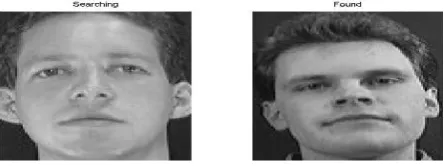
Fig 6: Correct face recognition result for ORL database
Fig 7: Incorrect face recognition result for ORL database
[image:5.595.318.541.434.501.2] [image:5.595.319.542.525.608.2]Fig 8: Correct face recognition result for IFD database
Fig 9: Incorrect face recognition result for IFD database
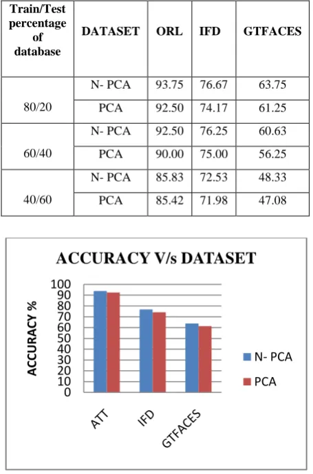
[image:6.595.316.536.73.479.2]The performance of the proposed feature extraction scheme (N-PCA) is compared with PCA in terms of percentage of recognition by varying the database ratio in training and testing and the results are presented in table 1 for all three ORL, IFD and GT-face database and also the accuracy v/s dataset graphs are plotted for different training and testing database ratio in figure 10, 11 and 12.
Table 1 Accuracy for N- PCA compared with PCA on different number of training and testing images Train/Test
percentage of database
DATASET ORL IFD GTFACES
80/20
N- PCA 93.75 76.67 63.75
PCA 92.50 74.17 61.25
60/40
N- PCA 92.50 76.25 60.63
PCA 90.00 75.00 56.25
40/60
N- PCA 85.83 72.53 48.33
PCA 85.42 71.98 47.08
Fig 11: Accuracy v/s Dataset for 60/40 ratio
Fig 12: Accuracy v/s Dataset for 40/60 ratio
6.
CONCLUSION
The face recognition system consists of two important steps, the feature extraction and the classification. This paper investigates the N-PCA function improvement over the principal component analysis (PCA) for feature extraction. The experiments carried out to investigate the performance of N-PCA by comparing it with the performance of the PCA. The analysis is done with ORL, IFD and GT-face dataset, the recognition performance for both algorithms are evaluated and the experimental results shows that N-PCA gives a better recognition rate. It is clear that the comparison shows that accuracy for PCA is 92.50%, 74.17 and 61.25%, while for N-PCA is 93.75%, 76.67% and 63.75 on ORL, IFD and GT-faces respectively. The promising results indicate that N-PCA can emerge as an effective solution to face recognition problem in future. And can give much better results if combined with techniques like curvelet transform.
7.
REFERENCES
[1] W. Zhao, R. Chellappa, P. Phillips, A. Rosenfeld, “Face recognition: a literature survey”, ACM Computing Surveys vol. 35, pp.399–458, December 2003.
[2] Daugman J. ,”Face and gesture recognition: Overview”, IEEE Trans. Pattern Analysis and Machine Intelligence, Vol. 19, No. 7, pp. 675-676,1997.
0 10 20 30 40 50 60 70 80 90 100
A
CCUR
A
CY
%
ACCURACY V/s DATASET
N- PCA
PCA
0 10 20 30 40 50 60 70 80 90 100
A
CCUR
A
CY
%
ACCURACY V/s DATASET
N- PCA
PCA
0 10 20 30 40 50 60 70 80 90 100
A
CCUR
A
CY
%
ACCURACY V/s DATASET
N- PCA
[image:6.595.53.281.402.747.2]survey”, Pattern Recognition, Vol. 25, No. 1, pp. 65-77,1992
[4] Valentin D., Abdi H., et al,”Connectionist models of face processing: a survey”, Pattern Recognition, Vol. 27, No. 9, pp. 1209-1230, 1994.
[5] Yang,M. H.,Kriegman, D., and Ahuja,N.,” Detecting faces in images: A survey ”, IEEE Trans. Pattern Analysis and Machine Intelligence, Vol. 24, No. 1, pp. 34-58, 2002..
[6] Pantic M. and Rothkrantz L.J.M., “Automatic analysis of facial expressions: the state of the art “, IEEE Trans. Pattern Analysis and Machine Intelligence, Vol. 22, No. 12, pp. 1424-1445, 2000.
[7] S.K.Singh, Mayank Vatsa, Richa Singh, K.K. Shukla, “A Comprative Study of Various Face Recognition Algorithms”, IEEE International Workshop on Computer Architectures for Machine Perception (CAMP), pp.7803-7970 ,5/03, 2003
[8] D. Beymer, “Face recognition under varying pose”, in IEEE Conf. on Comp. Vision and Patt. Recog., pages 756–761, 1994.
[9] M. Turk and A. Pentland, “Eigenfaces for Recognition,” J. Cognitive Neuroscience, vol. 3, no. 1, pp. 71-86, 1991. [10]K. J. Karande, S. N. Talbar, "Independent component analysis of edge information for face recognition," Image Processing Journal, vol. 3, no.3, pp.120-130, 2009.
[11]H. Zhang, W. Deng, 1. Guo, and 1. Yang, "Locality preserving and global discriminant projection with prior information," Machine Vision and Applications Journal, vol. 21, pp. 577-585, 2010.
[12]J. Li, B. Zhao, and H. Zhang, "Face recognition based on PCA and LDA combination feature extraction," 1st IEEE International Conference on Information Science and Engineering, pp. 1240-1243, 2009.
[13]K. Delac, M. Grgic, and S. Grgic, "Independent comparative study of PCA, ICA, and LDA on the FERET data set," Imaging Systems And Technology Journal, vol. 15, pp. 252-260, 2005.
[14]Abhishek Bansal, Kapil Mehta and Sahil Arora,” Face Recognition Using PCA & LDA Algorithms”, Second International Conference on Advanced Computing & Communication Technologies IEEE, 978-0-7695-4640-7/12, 2012.
[15]S. Haykin. Neural networks and learning machines. 3rd ed., Pearson, 2009.
[16]T. Pentland, B. Moghadam, and T. Stamer, "View based and modular eigenspaces for face recognition," IEEE Conference on Computer Vision and Pattern Recognition, pp. 84-91, 1994.
[17]M. Kirby, L. Sirovich, “Application of Karhunen–Loeve procedure for the characterization of human faces”, IEEE Transactions on Pattern Analysis and Machine Intelligence vol. 12, pp.103–108, 1990.
[18]M. A. Turk and A. P. Pentland, “Face recognition using eigenfaces,” in Proc. IEEE Computer Society Conf. Computer Vision and Pattern Recognition, Maui, Hawaii, pp.586-591, 1991.
[19]AT&T Laboratories Cambridge Database of faces. http://www.uk.research.att.com:pub/data/att_faces.zip.
[20]Vidit Jain, Amitabha Mukherjee. The Indian Face Database. www.cs.umass.edu/~vidit/IndianFaceDatabas, 2002.
[21]Georgia Tech face database developed at the Center for Signal and Image Processing at Georgia Institute of Technology.