WRL 92 2 pdf

(1)

A P R I L 1 9 9 2

WRL

Research Report 92/2

Observing

TCP Dynamics

in Real Networks

(2)

The Western Research Laboratory (WRL) is a computer systems research group that was founded by Digital Equipment Corporation in 1982. Our focus is computer science research relevant to the design and application of high performance scientific computers. We test our ideas by designing, building, and using real systems. The systems we build are research prototypes; they are not intended to become products.

There is a second research laboratory located in Palo Alto, the Systems Research Cen-ter (SRC). Other Digital research groups are located in Paris (PRL) and in Cambridge, Massachusetts (CRL).

Our research is directed towards mainstream high-performance computer systems. Our prototypes are intended to foreshadow the future computing environments used by many Digital customers. The long-term goal of WRL is to aid and accelerate the development of high-performance uni- and multi-processors. The research projects within WRL will address various aspects of high-performance computing.

We believe that significant advances in computer systems do not come from any single technological advance. Technologies, both hardware and software, do not all advance at the same pace. System design is the art of composing systems which use each level of technology in an appropriate balance. A major advance in overall system performance will require reexamination of all aspects of the system.

We do work in the design, fabrication and packaging of hardware; language processing and scaling issues in system software design; and the exploration of new applications areas that are opening up with the advent of higher performance systems. Researchers at WRL cooperate closely and move freely among the various levels of system design. This allows us to explore a wide range of tradeoffs to meet system goals.

We publish the results of our work in a variety of journals, conferences, research reports, and technical notes. This document is a research report. Research reports are normally accounts of completed research and may include material from earlier technical notes. We use technical notes for rapid distribution of technical material; usually this represents research in progress.

Research reports and technical notes may be ordered from us. You may mail your order to:

Technical Report Distribution

DEC Western Research Laboratory, WRL-2 250 University Avenue

Palo Alto, California 94301 USA

Reports and notes may also be ordered by electronic mail. Use one of the following addresses:

Digital E-net: DECWRL::WRL-TECHREPORTS

Internet: [email protected]

UUCP: decwrl!wrl-techreports

(3)

Observing TCP Dynamics in Real Networks

Jeffrey C. Mogul

April, 1992

Abstract

The behavior of the TCP protocol in simple situations is well-understood, but when multiple connections share a set of network resources the protocol can exhibit surprising phenomena. Earlier studies have identified several such phenomena, and have analyzed them using simulation or observation of contrived situations. This paper shows how, by analyzing traces of a busy segment of the Internet, it is possible to observe these phenomena in ‘‘real life’’ and measure both their frequency and their effects on performance. A TCP implementation might use similar techniques to support rate-based con-gestion control.

This Research Report is a slightly expanded version of a paper to appear in the Proceedings of

the SIGCOMM ’92 Conference on Communications Architectures and Protocols.

Permission to copy without fee all or part of this material is granted provided that the copies are not made or distributed for direct commercial advantage, the ACM copyright notice and the title of the publication and its date appear, and notice is given that copying is by permission of the Association for Computing Machinery. To copy otherwise, or to republish, requires a fee and/or specific permission.

(4)

(5)

List of Figures

Figure 1: TCP self-clocking 1

Figure 2: Self-clocking disrupted by ACK-compression 2

Figure 3: Sequence numbers vs. time for single connection 12

Figure 4: Instantaneous bandwidth distribution (same connection as fig. 3) 12

Figure 5: Partial packet trace (same connection as fig. 3) 14

Figure 6: Acknowledgement-number curves for ACK-compressed connections 15

Figure 7: Normalized curves (same traces as fig. 6) 15

Figure 8: Sensitivity of ACK-compression analysis (ACK-window size held con- 15

stant)

Figure 9: Sensitivity of ACK-compression analysis (minimum bandwidth held 16

constant)

Figure 10: Sensitivity of ACK-compression analysis (minimum ratio held con- 16

stant)

Figure 11: Distribution of connection durations 17

Figure 12: Distribution of packet counts 17

Figure 13: Distribution of connection lengths in bytes 17

Figure 14: Distribution of segment lengths 17

Figure 15: Distribution of average connection bandwidths 17

Figure 16: Distribution of median bandwidths 17

Figure 17: Distribution of lost segment counts 17

Figure 18: Distribution of out-of-order delivery counts 17

Figure 19: Loss interarrival times, all connections 19

Figure 20: Loss interarrival times, single connection 19

Figure 21: Loss interarrival times, differing connections 19

Figure 22: Connection with reduced average bandwidth associated with frequent 21

(8)

(9)

List of Tables

Table 1: Summary of traces 20

Table 2: Summary of detected events 20

(10)

(11)

1. Introduction

Although the TCP protocol has a relatively brief specification [14], and a functionally correct implementation can be as short as ten pages of source code, the dynamics of TCP in real net-works are not well understood. Real netnet-works in particular suffer from congestion; that is, con-tention for insufficient resources. While modern TCP implementations attempt to avoid or recover from congestion, they do this using delayed feedback mechanisms that exhibit complex behavior.

Most TCP implementations now in use include the congestion avoidance and control al-gorithms described by Van Jacobson [8]. Jacobson developed his alal-gorithms by observing the behavior of TCP implementations attempting to send data across a congested network. In these observations, the congestion was mostly due to a small number of connections, all sending data in the same direction via a single shared bottleneck link.

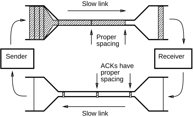
The essence of the congestion avoidance algorithms is the observation that data packets arrive at the receiving host at the rate that the bottleneck link will support. If the receiver’s ack-nowledgements (ACKs) arrive at the sender with the same spacing, then by sending new data packets at the same rate the sender can avoid overrunning the bottleneck link. It is by correctly exploiting this self-clocking property of TCP that congestion may be avoided (figure 1).

Sender Receiver

Proper spacing Slow link

Slow link

ACKs have proper spacing

[image:11.612.164.488.349.544.2]

The horizontal dimension represents time, and the shaded area is proportional to packet size (after [8]).

Figure 1: TCP self-clocking

Zhang, Shenker, and Clark [18] studied the slightly more complex case of a single link with TCP data flowing in both directions at once. Their simulations showed that several surprising phenomena could arise in such a situation, even when Jacobson’s algorithms were employed.

(12)

OBSERVINGTCP DYNAMICS INREALNETWORKS

1

the sender might be misled into sending more data than the network can accept, which could lead to congestion and loss of efficiency. (This analysis assumes that acknowledgement packets are small enough that queueing is the major cause of their delay.)

Sender Receiver

Proper spacing Slow link

Slow link ACKs have

improper spacing

[image:12.612.127.454.128.321.2]

Queueing causes burstiness

Figure 2: Self-clocking disrupted by ACK-compression

The insights of Zhang et al. were based on simulations. Two other studies have detected ACK-compression in actual implementations. Heybey [7] made traces of connections through the actual Internet, but these connections were set up specifically for the traces and might not have been representative. Wilder et al. [17] made traces of OSI TP4 connections, also in a testbed network. In all three cases, the results were analyzed by hand to detect interesting pat-terns, a technique that, while enlightening, cannot be applied to more complex situations.

This paper describes the results of a trace-based studies of large numbers of uncontrived con-nections through the Internet. These were obtained by monitoring the packets flowing in and out of a busy ‘‘gateway’’ system, widely used by sites all over the Internet for electronic mail and similar protocols. Tools were developed to automatically analyze the traces to detect ACK-compression and other interesting phenomena, and in some cases to show the correlation be-tween various phenomena in order to detect causal relationships.

1.1. Motivation

The primary motivation for these experiments was to determine if ACK-compression could actually be detected automatically, and to discover if it causes any problems. The experiments show that ACK-compression can indeed be detected automatically from packet traces, and that it does happen in real networks. They do not show any serious consequences of ACK-compression in today’s Internet, although this may be a result of our temporary inability to exploit the full bandwidth of the network.

1_{The terms sender and receiver will always be used with respect to the data packets, unless further qualified.}

(13)

Other phenomena besides ACK-compression, such as synchronization of losses between several connections, out-of-order packet delivery, and some forms of improper TCP behavior, can also be automatically detected from traces, as will be described in this paper.

A secondary question is whether, if ACK-compression does happen, there is anything that one could do about it. A TCP implementation could use techniques, similar to the trace-analysis tools described here, to infer when acknowledgements are being compressed. It could then limit the rate of outgoing packets to avoid overloading the bottleneck link.

The emphasis of the discussion in this paper will be on the methods and tools used to detect compression and related phenomena, rather than a broad study of the frequency of ACK-compression.

1.2. Related work

Timothy Shepard’s work on the problem of TCP packet trace analysis [16] extended the reper-toire of graphical methods for visualizing TCP traces, and described a way to quantify the bursti-ness of a connection. Automated detection of ACK-compression relies on a similar method (see section 2.3). Trevor Mendez [12] worked on the problem of identifying ‘‘pathological’’ TCP connections among the many connections captured in a long trace, concentrating on the retransmission behavior of TCP hosts.

Several studies have used traces to study the behavior of many simultaneous TCP connections in wide-area networks. Caceres et al. [1] analyzed traces to discover summary information about TCP connections, such as the number of packets transferred or the packet interarrival time. Vern Paxon [13] did similar analyses of a set of traces, and calculated the distribution of per-connection average bandwidths.

Much ongoing work on TCP behavior continues to use simulation, since trace analysis cannot capture all the aspects of a network (such as instantaneous window sizes and queue lengths). Recent studies include an analysis of traffic phase effects by Sally Floyd and Van Jacobson [6], Floyd’s analysis of connections through multiple congested routers [4], and the paper that describes ACK-compression [18].

Several simulation studies have identified other phenomena that might be visible to a trace-based analysis. For example, Shenker et al. [15] found in their simulations that when multiple connections use the same path, the packets from a given connection tend to be clustered together, rather than interleaved with those of other connections.

2. Methodology

Automatic detection of ACK-compression depends on successful approaches to several problems:

1. Choosing the monitoring point: The traces must be made of connections that have a reasonable likelihood of exhibiting ACK-compression.

(14)

3. Defining the phenomena: Unlike a simulation or a contrived experiment, in these trace it is impossible to observe the actual spacing of ACKs at both ends of the network path. Therefore, compression must be defined indirectly, based on ob-servable aspects of the trace.

The rest of this section discusses the approach taken to each of these issues, and similar issues in the detection of related phenomena.

Section 3 will discuss the tools that have been created to analyze the traces. These tools must solve two problems:

1. Detecting the phenomena in the traces: Algorithms must be created to analyze the traces to detect when the defined phenomena are present.

2. Visualizing the results: Because there may be thousands of connections and events represented in a trace, the results of the analysis should be presented in a form that allows easy and rapid understanding.

2.1. Choosing the monitoring point

The ideal site for obtaining these traces would be one through which passes many TCP con-nections, between a wide variety of TCP hosts throughout the Internet, and which transfer more than just a few packets’ worth of data at a time. (If the connections are too short, they will not generate enough ACKs to allow compression.) Also, the traces should be made as close as pos-sible to the end-point of these connections, since it is only there that the final spacing of ACKs may be observed.

These criteria suggest monitoring at a major ‘‘gateway’’ complex, one which makes long TCP connections with sites all over the Internet. Fortunately, the author has easy access to the DECWRL gateway, operated by the Network Systems Laboratory of Digital Equipment Cor-poration. This site exchanges over 16,000 electronic mail messages every day, as well as thousands of USENET ‘‘news’’ articles. The gateway also includes a popular ‘‘anonymous FTP’’ site, from which several thousand files are retrieved each day.

Although most mail messages are too short to give rise to interesting TCP behavior, the gateway also provides an ‘‘FTP-by-mail’’ facility that produces about 150 relatively lengthy messages every day. News articles are also short, but they are sent in batches via the NNTP [9] protocol, and so give rise to long connections. Many FTP transfers involve large files.

Since the traces are being made at one endpoint of the TCP connections, ACK-compression can only be observed on those connections that carry bulk data away from the gateway complex. This halves the number of potentially interesting ACK-compression events in the trace.

(15)

During the initial phases of this study, a question arose as to whether the TCP window sizes in common use would be large enough to stimulate ACK-compression. Many hosts use window sizes of just 4k bytes, which might be too small to elicit the phenomenon, but quite a few hosts now use 16k-byte windows. (In our traces, at least half of the connections used windows of 16k bytes or more.) In any case, although the NSFNet can transport 1500-byte datagrams to many sites, most TCP hosts use a segment size of 512 bytes in order to avoid possible fragmentation; this means that even with a relatively small window size of 4k bytes, up to eight packets may be in transit at once. Our results show that for whatever reason, the issue of window size has not been an impediment to the detection of ACK-compression.

One advantage of making the traces at an endpoint site, rather than at a backbone, is that by definition that site is a party to all of the connections traced. This simplifies the issue of obtain-ing permission, but it would be unethical (and perhaps illegal) to monitor the content of the con-nections without the permission of both parties [2]. The traces therefore contain only packet header data, and not anything that could be used to compromise the privacy of the messages traced.

2.2. Obtaining traces

The traces were obtained by ‘‘promiscuous-mode’’ monitoring of 10 Mbit/sec Ethernet net-works. This passive monitoring technique eliminates any effect that the trace-gathering process might have on the connections being traced. It also means that no changes need be made to the hosts whose connections are traced.

2.2.1. Tracing environment

The trace-gathering program runs on any ULTRIXversion 4.2 system, and for these experi-ments was run on DECstation 3100 workstations. During the traces, little additional activity was present on the trace-gathering system. Trace files were written to disk for later analysis, rather than being transferred over the network in real-time (which might have affected the net-work being traced).

Some simple arithmetic will demonstrate that to detect ACK-compression, the traces must contain high-resolution timestamps. For example, suppose that a TCP connection is using 1500-byte packets over a path with an effective bandwidth of 10 Mbit/sec. This means that properly-spaced ACKs will be sent approximately 1.2 msec apart. A timestamp resolution coarser than about half of that will make some properly-spaced ACKs appear to be compressed together, since they will arrive during the same ‘‘tick.’’

ULTRIX normally updates its timebase just 256 times per second, yielding a resolution of about 4 msec. To obtain better timestamps, the ULTRIXkernel used on the tracing systems was modified to use a 4096 hz timebase, yielding a resolution of about 244 usec. Additionally, the traces record the length of each packet; this allows some subsequent ‘‘decompression’’ of time-stamps because the minimum spacing between two packets, as they were transmitted on the monitored Ethernet, can be calculated from their lengths (see section 3).

(16)

nsec, although the usable resolution is not quite this good because the timestamps are applied by the kernel and so are smeared by the latency of the interrupt-handling code.

2.2.2. Creation of a trace file

The tracing program is conceptually quite simple. The IP header of each TCP packet received is parsed to obtain source and destination addresses, and the TCP header is parsed to obtain the source and destination ports, the sequence and acknowledgement numbers, the flags, and the window size.

Since the addressing information is repetitive, the program maintains a map from TCP address tuples (the two IP addresses and the two TCP port numbers) to a compact connection identifier. (At any one time, this is enough information to uniquely identify a connection, but during the life of a trace there may be several connections that reuse the same address tuple. In a post-processing phase, it is easy to split the trace up into distinct connections, because the TCP protocol has rules to prevent any confusion.) Whenever a new connection is seen, the tracing program emits a record containing the new connection ID and the associated addressing infor-mation. For each packet received, the program emits a record containing the timestamp, connec-tion ID, and the non-address fields from the TCP header.

Note that the connection ID identifies one direction of packet flow; TCP connections are al-ways full-duplex, and the relationship between the two half-connections can be recreated in a post-processing phase.

The connection ID mapping is done using a hash table, with 1024 hash slots each pointing to a chain of entries. A simple hash function on the address information distributes the entries remarkably evenly, with no chain more than three times longer than the average. A ‘‘one-behind’’ cache bypasses the hash table lookup whenever two or more successive packets belong to the same connection.

In spite of the compression of address information, the trace files are still quite bulky. A file representing a trace of 1 million packets requires just under 32 Mbytes of disk space. In order to avoid cluttering the trace with irrelevant information, the trace program can be made to ignore packets between pairs of ‘‘local’’ hosts, where ‘‘local’’ refers to a host whose address is the same as the tracing host, when compared under a given bit mask. For traces made at the DECWRL gateway site, this mask covered the IP network number; for traces made internal to Digital’s IP network, the mask covered the network and subnet numbers.

2.2.3. Potential problems with passive monitoring

(17)

In the traces made for this paper, the trace-gathering system was able to keep up with the traffic. In no case were even 0.2% of the packets dropped. While it is impossible to tell if the dropped packets conceal an unusually high number of ACK-compression events, it is unlikely that this is the case.

Another problem with passive monitoring is that it occasionally accepts packets with check-sum errors. While it is theoretically possible to have the tracing program check the header checksums on each packet, in practice this would so slow the program that it would certainly lose far too many packets. (Checksumming is now considered to be the most expensive part of processing a TCP packet [3].) Statistics kept by the gateway machines show that packets with bad checksums, while present, are quite rare. The danger for this experiment is that a damaged packet might give rise to a trace record that confuses the analysis tools. The tools take some care to ignore connections that contain bizarre packets, but it is possible that corruption of a few bits could cause false conclusions to be drawn on rare occasions.

2.3. Defining the phenomena

When ACKs are observed arriving at the end of their transit through the Internet, it is impos-sible to know precisely how they were spaced when they were sent. (When ACKs are observed near the receiver, we can tell their spacing, but we then do not see them arriving at the other end and so can say nothing at all about their possible compression.) This means that the trace analysis tools must infer ACK-compression from indirect evidence. Choosing a satisfactory definition is thus key to the utility of the analysis, and proved to be somewhat difficult.

What we can observe, by looking at the number of bytes acknowledged by a set of ACKs and the time spacing between them, is the apparent network bandwidth that these ACKs promise to the sender. (This is precisely the information that the sender uses to meter out its data traffic.) This is called the ‘‘instantaneous ACK bandwidth’’ of the observed ACKs. We want to know if this value is much higher than the actual bandwidth of the path, which would indicate that ACK-compression has occurred.

Another thing we can observe is the actual progress of the connection over intervals long com-pared to the TCP window size. Clearly, the bandwidth obtained during such an interval cannot be higher than the actual available bandwidth. If we can measure this ‘‘true’’ bandwidth, then we can define ACK-compression as occurring when the instantaneous ACK bandwidth is sig-nificantly greater than the true bandwidth.

The simplest way of calculating the bandwidth of a connection, given a trace of all its ACKs, is to divide the total number of bytes acknowledged by the total time required. Unfortunately, most connections do not proceed at a steady rate, and so this average rate is almost always far too small.

Plots of ACK-value versus time for actual TCP connections show phases of relatively steady progress (diagonal lines) interspersed with dead periods (horizontal lines). Clearly, what we want is to ignore the dead periods when computing the true bandwidth.

(18)

x-axis of these plots shows the number of bytes carried in a packet divided by the time since the previous packet; the y-axis shows the total number of bytes transferred at a given instantaneous bandwidth. Since the dead periods transfer few or no bytes, they contribute little to the distribu-tion, and the peaks of the distribution show the approximate true bandwidths attained during various phases of the connection.

If there is one main peak to this distribution, we can find its approximate position on the x-axis by taking the median of the distribution. This provides a simple, automatic mechanism for estimating the true bandwidth of a connection that transfers a lot of data over a stable path.

It is possible that if the connection’s rate is actually limited by something external to the net-work, such as a disk drive on one of the end systems, this mechanism will underestimate the true bandwidth. There is not much one can do about this, if the information in the traces is all that is available. One could in principle set up ‘‘probe connections’’ along the paths followed by inter-esting connection, and attempt to measure the available bandwidth; this is not always possible, and was not done for this study. Anyway, the results suggest that the alleged ACK-compression events are often real, since they are often associated either with subsequent segment loss or with periods of reduced throughput. If they were a consequence of an underestimate of the available bandwidth, one would expect to see them associated with periods of increased throughput.

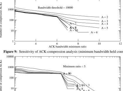
Some additional filtering reduces falsely-detected ACK-compression. First, we can insist that a compression event last for at least a certain number of packets (i.e., the ACK-bandwidth is measured over a window of A packets, where A might be greater than the minimum of two.) Second, we can insist that the ACK-bandwidth exceed the estimated true bandwidth by a ratio R (such as 5 or 10) in order to correct for serious underestimates of this value. Third, we can insist that a compression event show a certain minimum ACK-bandwidth B, in order to omit connec-tions that don’t actually transmit much data. This threshold should be set slightly above an es-timate of the lowest link-bandwidth in the network, since setting it much higher could hide ACK-compression on low-bandwidth links.

2.3.1. Segment loss and out-of-order delivery

We would like to be able to detect TCP segment losses since these are the main consequence of improper segment spacing. Since we cannot directly know when a segment has been lost, we have to infer segment loss from the observed retransmission of a segment. Note also that if a segment flowing into the monitored site is lost, we will never know this because even if we receive a retransmitted copy, without having seen the original we will not recognize the retransmission as such. In other words, we can only detect retransmissions on connections that transfer data out of the monitored site. Fortunately, since we can detect ACK-compression on only these same full-connections, it should be possible to detect correlations between ACK-compression and segment loss, if the correlations exist.

We define retransmission to have occurred if we see a segment whose sequence number lies within the ranges of bytes transmitted by another segment.

(19)

3. Analysis Tools

Once the traces are made, they must be analyzed to detect the phenomena of interest. Analysis is done offline, because a connection cannot be analyzed until it is complete, and be-cause on-line analysis would interfere with packet-gathering and be-cause packet loss. Many kinds of off-line analysis can be applied to a single trace file.

2

Several different primary analyses can be applied to the connections in a trace:

•Aggregate statistics: For each connection, we compute the total duration, number

of bytes sent (i.e., the net change in sequence number), number of bytes acknowl-edge (the net change in acknowlacknowl-edgement number), and the median ACK-bandwidth.

•ACK-compression: Given parameter values for the ACK-compression detection

window, minimum ACK-bandwidth, and minimum ratio to the median, we find those ACK packets that appear to have been compressed.

•Segment retransmission, out-of-order delivery: By examining sequence

num-bers, packet lengths, and timestamps we discover those segments that have been retransmitted or have arrived out of order.

These primary analyses can then be combined in several ways (for example, to find correla-tions between ACK-compression and segment loss) and the results then plotted.

3.1. Data structures to support analysis

Each analysis tool starts by reading a saved trace file. An in-memory database is built up from the connection and packet-header records in the file. For each new connection, a connection record is created and inserted into a hash table (for rapid location based on the compact connec-tion ID.) Each packet-header record is stored in a header record, and added to the end of a linked-list of headers attached to the appropriate connection record. Since the trace file is or-dered by packet arrival time, the lists of headers are also time-oror-dered.

During this process, the timestamps being read in are checked to make sure that they are no closer together than the minimal possible spacing on an Ethernet. (If traces were made on a different LAN, such as FDDI, this calculation would have to be modified.) If one header record follows the previous one with a timestamp difference shorter than would be possible based on the length of the previous packet, the timestamp of the new record is increased accordingly.

Another problem with the raw trace data is that while at any given time the TCP address tuple uniquely identifies a connection, once a connection is terminated the same address tuple may be reused shortly thereafter. Since the sequence numbers from the two connections bear no relation to each other, in order to make sense of the sequence numbers the connections must be separated. This is done by searching for tell-tale signs of the end or beginning of a connection: packets bearing the FIN or SYN flags, or large jumps in the sequence or acknowledgement

num-2_{Remember that the term ‘‘connection’’ refers in this case to a half-duplex, one-way packet flow. An actual TCP}

(20)

bers. The largest legal jump in a TCP sequence number is the maximum window size of 64k bytes. Any jump larger than this suggests that a new connection has been made, although it is also possible that the trace-gathering program has either dropped a bunch of packets, or has ac-cepted a corrupted packet. In either case, since we are lacking sufficient information to analyze the entire connection, splitting into two connections avoids the problem of data integrity.

Once in a while, a trace contains data that just doesn’t make sense. For example, the final sequence or acknowledgement number is much lower than the initial value. While this could occur because of sequence-number wraparound, it can also be due to corrupted data, so the tools simply discard the entire connection in this case.

The in-memory database of connection and header records can be quite large. Each header record in its in-memory form contains 36 bytes; this could be reduced somewhat with compres-sion techniques, but that would make the whole process run slower. As a result, a trace of 1 million packets requires somewhat more than 36 Mbytes of virtual address space, and since the locality of reference to this database is poor, the analysis must be carried out on a machine with at least that much real memory. The largest machine available for these experiments, a DECsta-tion 5000/200, has 480 Mbytes of RAM, so traces of up to about 10 million packets could have been analyzed, but such traces would have required a lot of disk storage.

The running time of the analysis programs depends heavily on the cost of reading the trace file and constructing the internal database. On the systems with 480 Mbytes of RAM, the file system’s buffer cache can hold an entire trace file of 1 million packets, so the cost of an analysis depends entirely on CPU speed. On the DECstation 5000/200, the simplest analysis (not requir-ing the computation of median ACK-bandwidths) takes about 30 seconds, 20% of which is spent in the read() system call and 30% of which is spent correcting the timestamps and inserting header records into the database. (The more complex analyses take several minutes, because the algorithm used for finding medians is quite crude.)

3.2. Detecting the phenomena in the traces

Once all of the connection and header records have been created, passes can be made over the entire database, or over the header record list for a specific connection.

3.2.1. Detecting ACK-compression

If the analysis requires detection of ACK-compression in a connection, the first pass computes the median of the instantaneous ACK-bandwidths. First, the program calculates the instan-taneous ACK-bandwidth for each packet with the ACK flag set; this is computed by dividing the difference in acknowledgment numbers between successive ACK packets by the time elapsed between their reception. The program then records the instantaneous bandwidth samples in an array, and sorts the array. Finally, it locates the median value, weighted by the number of bytes acknowledged at each rate. (A more sophisticated median-finding algorithm might reduce the time required for an analysis, but since it takes less than 90 seconds to analyze a 1-million packet trace, this has not been a problem.)

(21)

bandwidth is calculated over the ‘‘ACK window size’’ A, specified as a parameter to the analysis. For example, if A = 3, then the ACK-bandwidth is calculated between an ACK-packet and the third following ACK-packet. If the instantaneous bandwidth exceeds the connection’s median by a specified ratio R, and also exceeds a specified minimum value B, the header records in the window are flagged as being ‘‘compressed.’’

3.2.2. Detecting segment retransmission and out-of-order delivery

A separate pass over the header record list is made to find retransmitted TCP segments. During this pass, an array is created containing an entry containing the sequence number and length of each packet, a serial number indicating the order of reception, and a back-pointer to the associated header record.

This array is then sorted, using the sequence number as the primary key, the length as the secondary key, and the reception order as the tertiary key. One more pass over the sorted array suffices to detect retransmissions and out-of-order delivery:

•If an array entry’s sequence number falls within the range of bytes carried by a pre-vious packet, then the entry is a retransmission. (We ignore packets with SYN set, since typically a lot of these are sent during an attempt to make a connection with a dead host.) The earlier packet is flagged as having been lost, and the later packet is flagged as a retransmission.

•During the pass over the sorted array, we can also detect and flag packets delivered out of order, since these are ones whose reception order is earlier than their predecessor in the array (which is sorted by sequence number), if the predecessor is not a retransmission.

4. Visualizing the results

Once the automated analysis has found connections with anomalous behavior, one needs some way to visualize the results. Visualization methods for these experiments can be divided into those showing just one connection, and those that show all (or a subset) of the connections. Also, the methods can be divided into graphical presentations, which abstract a lot of the details of individual packets, and textual presentations, which provide detailed insights but do not easily reveal interesting patterns. All four combinations of scope and presentation are useful.

4.1. Graphical presentation of single connections

(22)

An example of one such plot is shown in figure 3. The sequence-number plot is a solid line, and the acknowledgement-number plot is a broken line. (This connection starts with a period of about 25 seconds during which few bytes are transferred.) Regions of ACK-compression are bounded by ‘‘+’’ symbols, segment losses are marked with ‘‘X’’ symbols. In color media, these symbols can be made much easier to distinguish, and color may also be used to highlight regions of the curve suffering from ACK-compression.

Examination of such plots quickly provides insight into such issues as the actual underlying bandwidth of the connection (from the slope of the diagonal segments of the curve), and the relationship between compression and overall performance. For example, if ACK-compression were deleterious, one would expect to see decreases in the slope, or segment loss events, shortly after an instance of ACK-compression. In figure 3, this seems to be the case; shortly after the first ACK-compression event, an entire window-full of packets is sent in a brief interval, and all of these packets are lost.

0 20 40 60 80 100

time (seconds since start of connection) 0

100000

20000 40000 60000 80000

SEQ number (bytes)

[image:22.612.59.484.267.437.2]

median ACK-bw = 27144 bytes/sec

Figure 3: Sequence numbers vs. time for single connection

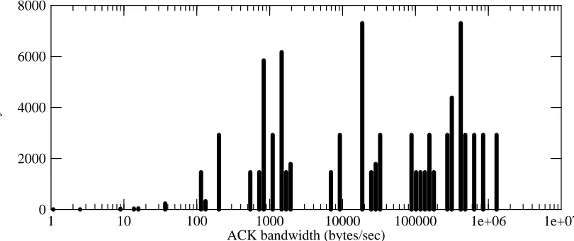
Following Shepards’s approach [16], we can also plot the distribution of instantaneous ACK bandwidths, as in figure 4. This more directly reveals the underlying network bandwidth, if one assumes that the spikes near 1 Mbyte/sec are the result of ACK compression rather than an in-dication of the true bandwidth.

1 10 100 1000 10000 100000 1e+06 1e+07

ACK bandwidth (bytes/sec) 0

8000

2000 4000 6000

Total # bytes ACKed

[image:22.612.72.477.528.698.2]

(23)

4.2. Textual presentation of single connections

Sometimes the Jacobson plots do not show enough detail to understand the precise dynamics of a connection. In this case, it helps to look at a trace of the individual packets of a connection, showing the exchange of packets in both directions in the correct time sequence.

(Because TCP is not a lock-step protocol and the hosts involved may be separated by a long-delay path, the actual ordering of packets may depend on where one observes it. For example, if host A and host B are 100 milliseconds apart, and host A sends an acknowledgment packet to host B 10 milliseconds after host B sends a data packet to host A, an observer near host A will see the packets in the opposite order from an observer near host B. This ‘‘relativistic effect’’ rarely appears.)

Packet traces can be difficult to analyze, even for an expert, but some help can be provided. For example, although TCP’s 32-bit sequence numbers are hard to deal with directly, the

tcpdump program [11] reports not the absolute sequence numbers but the relative value since the

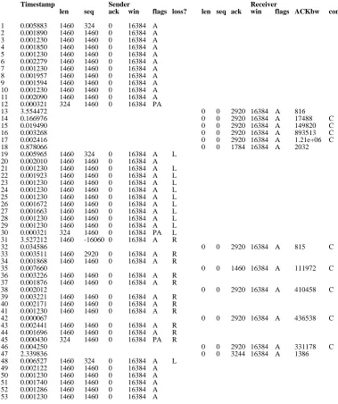
first observed packet of a connection. It seems even more useful to report the difference in sequence numbers between two successive packets, because that can be directly related to the amount of data transferred. Also, by showing the two halves of a connection in side-by-side columns, following Shepard’s example [16], one gets a picture of the time-ordering of the pack-ets. By displaying relative instead of absolute timestamps, the short-term dynamics are made apparent. Figure 5 shows part of the same connection as figure 3, packet-by-packet.

In figure 5, the sender’s packets are shown on the left, and the receiver’s on the right. The first column numbers the packets, for convenience in explanation. The second column shows the timestamp, in seconds since the preceding packet. The next four columns show the data length (exclusive of headers), the increment in sequence and acknowledgment numbers, the offered window size, and the TCP flag bits. The final column on the sender’s side marks lost or retransmitted packets (with ‘‘L’’ or ‘‘R’’, respectively). On the receiver’s side, the sixth column shows the instantaneous ACK-bandwidth, and the final column marks compressed packets (with ‘‘C’’).

On lines 1 through 12, we see the series of data packets being sent, then a burst of ACKs (lines 13 through 18). The last column shows that some of these ACKs (lines 14 through 17) appear to

3

have been compressed , and indeed most of the packets in the next burst (lines 19 through 30) are lost (marked with ‘‘L’’). After a 3.5 second timeout, the sender realizes this and enters a slow-start phase (starting with line 31), which revives the transfer of data.

4.3. Graphical presentation of multiple connections

Although the sequence-number curve in figure 3 is useful for displaying one connection, an entire trace might contain thousands of connections, and it would be impossible to study all those curves. There is a variety of more useful ways to display the aggregate behavior of many con-nections.

3_{All the ACKs in a compression event are marked with ‘‘C,’’ including those which arrive first and thus whose}

(24)

Timestamp Sender Receiver

len seq ack win flags loss? len seq ack win flags ACKbw comp?

1 0.005883 1460 324 0 16384 A 2 0.001890 1460 1460 0 16384 A 3 0.001230 1460 1460 0 16384 A 4 0.001850 1460 1460 0 16384 A 5 0.001230 1460 1460 0 16384 A 6 0.002279 1460 1460 0 16384 A 7 0.001230 1460 1460 0 16384 A 8 0.001957 1460 1460 0 16384 A 9 0.001594 1460 1460 0 16384 A 10 0.001230 1460 1460 0 16384 A 11 0.002090 1460 1460 0 16384 A 12 0.000321 324 1460 0 16384 PA

13 3.554472 0 0 2920 16384 A 816

14 0.166976 0 0 2920 16384 A 17488 C

15 0.019490 0 0 2920 16384 A 149820 C

16 0.003268 0 0 2920 16384 A 893513 C

17 0.002416 0 0 2920 16384 A 1.21e+06 C

18 0.878066 0 0 1784 16384 A 2032

19 0.005965 1460 324 0 16384 A L 20 0.002010 1460 1460 0 16384 A 21 0.001230 1460 1460 0 16384 A L 22 0.001923 1460 1460 0 16384 A L 23 0.001230 1460 1460 0 16384 A L 24 0.001230 1460 1460 0 16384 A L 25 0.001230 1460 1460 0 16384 A L 26 0.001672 1460 1460 0 16384 A L 27 0.001663 1460 1460 0 16384 A L 28 0.001230 1460 1460 0 16384 A L 29 0.001230 1460 1460 0 16384 A L 30 0.000321 324 1460 0 16384 PA L 31 3.527212 1460 -16060 0 16384 A R

32 0.034586 0 0 2920 16384 A 815 C

33 0.003511 1460 2920 0 16384 A R 34 0.001868 1460 1460 0 16384 A R

35 0.007660 0 0 1460 16384 A 111972 C

36 0.003226 1460 1460 0 16384 A R 37 0.001876 1460 1460 0 16384 A R

38 0.002012 0 0 2920 16384 A 410458 C

39 0.003221 1460 1460 0 16384 A R 40 0.002171 1460 1460 0 16384 A R 41 0.001230 1460 1460 0 16384 A R

42 0.000067 0 0 2920 16384 A 436538 C

43 0.002441 1460 1460 0 16384 A R 44 0.001696 1460 1460 0 16384 A R 45 0.000430 324 1460 0 16384 PA R

46 0.004250 0 0 2920 16384 A 331178 C

47 2.339836 0 0 3244 16384 A 1386

[image:24.612.86.465.70.522.2]

48 0.006527 1460 324 0 16384 A L 49 0.002122 1460 1460 0 16384 A 50 0.001230 1460 1460 0 16384 A 51 0.001740 1460 1460 0 16384 A 52 0.001286 1460 1460 0 16384 A 53 0.001230 1460 1460 0 16384 A

Figure 5: Partial packet trace (same connection as fig. 3)

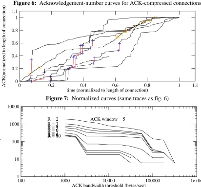
Since we have an algorithm to detect connections that display ACK-compression, if there are only a few such connections it is feasible to overlap their acknowledgement-number curves. Figure 6 shows those curves for one trace; figure 7 shows the same curves, normalized for both the duration and byte-count of each connection.

(25)

0 100 200 300 400 500 600 700

250000

50000 100000 150000 200000

ACK number (bytes)

66 111

190 953

1249

1285 1766

[image:25.612.100.520.68.236.2]

2582

Figure 6: Acknowledgement-number curves for ACK-compressed connections

0 0.2 0.4 0.6 0.8 1 1.1

time (normalized to length of connection) 0

1.1

0.2 0.4 0.6 0.8 1

ACK(normalized to length of connection)

Figure 7: Normalized curves (same traces as fig. 6)

100 1000 10000 100000 1e+06

ACK bandwidth threshold (bytes/sec) 1

10000

10 100 1000

Number of compressed ACKs

R = 2 R = 3 R = 4 R = 5 R = 6 R = 7 R = 8 R = 9 R = 10

ACK window = 5

Figure 8: Sensitivity of ACK-compression analysis (ACK-window size held constant)

[image:25.612.104.516.244.628.2]

(26)

2 4 6 8 10 12

ACK bandwidth minimum ratio 1

10000

10 100 1000

Number of compressed ACKs

A = 2 A = 3 A = 4 A = 5 A = 6

[image:26.612.68.474.67.236.2]

A = 7 A = 8 A = 9 A = 10 Bandwidth threshold = 10000

Figure 9: Sensitivity of ACK-compression analysis (minimum bandwidth held constant)

1000 10000 100000 1e+06 1e+07

ACK bandwidth threshold (bytes/sec) 1

10000

10 100 1000

Number of compressed ACKs A = 2

A = 3 A = 4 A = 5 A = 6 A = 7 A = 8 A = 9

A = 10

[image:26.612.61.480.75.384.2]

Minimum ratio = 5

Figure 10: Sensitivity of ACK-compression analysis (minimum ratio held constant)

4

through 18) . Some of these are useful for providing a context for understanding the important of ACK-compression. The data plotted in figure 13 show that most connections transfer only a few thousand bytes (about 75% of the connections transfer less than 10k bytes), and so are un-likely to suffer from ACK-compression. Figures 17 and 18, respectively, show that very few connections suffer from segment retransmission or out-of-order delivery.

4_{To avoid expanding the vertical scale, figures 13 through 18 do not include samples for which the x-axis value is}

(27)

1 10 100 1000 10000 Connection duration (seconds)

0 1000 200 400 600 800

Number of connections

1 10 100 1000 10000 100000 1e+06 Average ACK Bandwidth (bytes/sec)

0 100 20 40 60 80

[image:27.612.166.529.65.667.2]

(832 connections with zero bandwidth)

Figure 11: Distribution of Figure 15: Distribution of average

connection durations connection bandwidths

1 10 100 1000 10000 Packet count 0 1000 200 400 600 800

1 10 100 1000 10000 100000 1e+06 Median ACK bandwidth (bytes/sec)

0 80

20 40 60

(837 connections with zero bandwidth)

Figure 12: Distribution of Figure 16: Distribution of

packet counts median bandwidths

1 10 100 1000 10000 100000 1e+06 Total bytes transferred

0 500 100 200 300 400

(1098 connections sending zero bytes)

1 10 100 1000

Number of retransmitted segments 0 120 20 40 60 80 100

(2526 connections with no retransmissions)

Figure 13: Distribution of connection Figure 17: Distribution of

lengths in bytes lost segment counts

1 10 100 1000 10000 Data bytes per segment

0 12000 2000 4000 6000 8000 10000

Number of segments

(34544 zero-length segments)

1 10 100 1000

Number of segments delivered out of order 0 100 20 40 60 80

(2757 connections with no out-of-order segments)

Figure 14: Distribution of Figure 18: Distribution of

[image:27.612.334.535.69.595.2]

(28)

4.4. Statistical analyses of multiple connections

It is interesting to ask whether there are frequent correlations between ACK-compression and segment losses. One could obtain timestamps for all the compression events and all the loss events in a trace, and try to establish if a statistically significant correlation exists. A more direct approach is to look at each full connection that experiences both compression and segment loss, and analyze the timestamps to see if there is a causal relationship between compression and loss.

Inference of a causal relationship can be done in a number of ways. One would be to assume that any packets lost in the next TCP window after a compression event are caused by that event, but it is not always possible to be sure that those packets were not sent before the compressed ACKs arrived at the sender. Another approach is to measure the time between an ACK-compression event and the next segment loss event. One could then compare this interval to an estimate of the round-trip time. Even simpler is to see if the interval is small compared to the median interval between loss events; this last method shows that in many cases there does seem to be a causal relationship.

For example, in one trace made on Digital’s internal network, 63 connections experienced at least one loss event subsequent to a compression event, and in 42 of those cases the time be-tween a compression event and a subsequent loss event was less than the median time bebe-tween losses. (These intervals between reception of compressed ACKs and transmission of a lost seg-ment are typically on the order of several milliseconds or tens of milliseconds.)

Simulations by Shenker et al. [15] suggested that when multiple TCP connections are sharing a congested resource, their congestion-recovery behavior could become synchronized, with each connection loosing a packet at each congestion epoch. The timestamped segment-loss events obtained from traces could, in principle shed some light on this effect. Synchronized segment loss can be detected by making an array of all the loss events in a trace, sorting this array by timestamp, and then looking for losses from different connections that occur within no more than a specified interval. (The choice of this interval is an arbitrary parameter, because of course no two packets can be lost at precisely the same instant.)

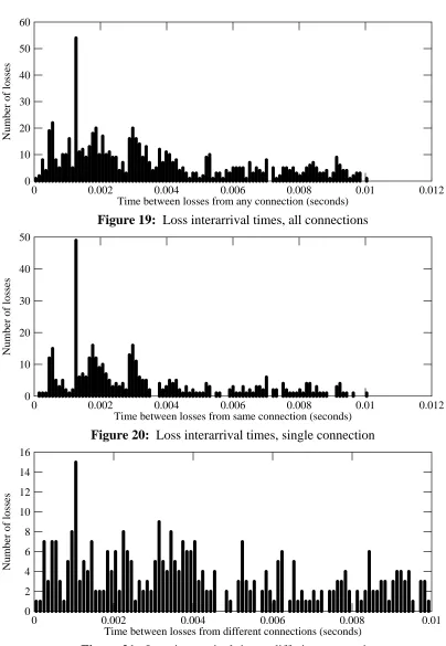
In the trace mentioned above, out of 5142 losses, in 287 cases losses from two or more con-nections occurred less than 10 msec apart. It is not clear, however, if this reflects a statistically significant correlation between losses from multiple connections. Figures 19, 20, and 21 show for this trace the distribution of interarrival times (respectively) for packet losses among all con-nections, for two losses encountered by a single connection, and for two losses where second occurs to a different connection than the first. The spikes at 460 usec and 1200 usec reflect the back-to-back transmissions of 576-byte and 1500-byte packets, respectively: when TCP sends a burst of packets, the entire burst is likely to be lost as a group. Aside from these spikes, the data might reflect a Poisson distribution, but it may be too noisy to demonstrate a clear correlation between losses from differing connections.

5. Summary of Experiments

(29)

dura-OBSERVINGTCP DYNAMICS INREALNETWORKS

0 0.002 0.004 0.006 0.008 0.01 0.012

Time between losses from any connection (seconds) 0

60

10 20 30 40 50

Number of losses

Figure 19: Loss interarrival times, all connections

0 0.002 0.004 0.006 0.008 0.01 0.012

Time between losses from same connection (seconds) 0

50

10 20 30 40

Number of losses

Figure 20: Loss interarrival times, single connection

0 0.002 0.004 0.006 0.008 0.01

Time between losses from different connections (seconds) 0

16

2 4 6 8 10 12 14

[image:29.612.113.517.51.636.2]

Number of losses

Figure 21: Loss interarrival times, differing connections

tions are in seconds. ‘‘Dropped packets’’ are those discarded because the monitoring system could not keep up; there is no way to know precisely what kinds of packets were dropped.

(30)

ID Site Date/Time Duration Packets Connections Dropped pkts

[image:30.612.108.468.71.179.2]

I1 Internal 2 Jan 92, 13:21 1079 100K 2868 0 I2 Internal 2 Jan 92, 10:21 7099 1M 17595 158 I3 Internal 3 Jan 92, 10:14 5518 1M 14635 88 E1 External 2 Jan 92, 10:19 8227 1M 25907 880 E2 External 3 Jan 92, 10:17 7029 1M 24498 1149

Table 1: Summary of traces

Tables 2 and 3 summarize the number of lost segments detected. They also show the number of ACK-compression events and causally-correlated segment-loss events for two different com-binations of ACK-compression detection parameters.

ID Losses Compressions Correlations ID Losses Compressions Correlations

I1 5142 388 10 I1 5142 0 0

I2 19321 2076 42 I2 19321 156 1

I3 10443 2832 33 I3 10443 168 1

E1 19778 2732 95 E1 19778 240 6

E2 18491 5124 144 E2 18491 264 12

ACK-window A = 3 ACK-window A = 5

Bandwidth threshold B = 10Kbytes/sec Bandwidth threshold B = 100Kbytes/sec Minimum ratio to median R = 5.0 Minimum ratio to median R = 10.0

Table 2: Summary of detected events Table 3: Summary of detected events

As a check on the reliability of the method that looks for cause-effect relationships between ACK-compression and segment loss, plots were made of the 12 connections in Trace E2 iden-tified as having such correlations even with the stricter parameters used in table 3. Inspection of these plots suggests that in about half of the cases, a causal relationship is likely, and could not be ruled out in several other cases.

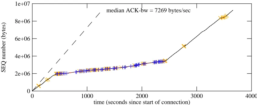
The possibility exists that some of the detected instances of ACK-compression are actually periods during which the available bandwidth is much higher than normal. This is probably true in some cases, but there are definitely connections for which the reverse is true. Figure 22 shows a connection for which there is a period with many ACK-compression events. During this period, the average bandwidth is far lower than it is during other phases of the connection, which do not exhibit ACK-compression.

[image:30.612.61.522.256.429.2]

(31)

0 1000 2000 3000 4000

1e+07

2e+06 4e+06 6e+06 8e+06

SEQ number (bytes)

[image:31.612.94.516.65.238.2]

median ACK-bw = 7269 bytes/sec

Figure 22: Connection with reduced average bandwidth

associated with frequent ACK-compression

6. Future work

6.1. Application to congestion avoidance

Since ACK-compression and subsequent packet loss occurs even on networks that are believed to be uncongested over the long term, this implies that portions of the Internet ex-perience temporary congestion over short periods. These periods may in fact be shorter than the response time of feedback-based congestion-avoidance schemes, which means that some form of rate-based congestion avoidance may be required. While most proposals for rate-based schemes have the network provide explicit rate-limit information to the end-hosts, it may be possible for an end-host to infer the true available bandwidth and thus set its own rate limit. In effect, the end-host could use the ACK-compression detection methods described in this paper to avoid being misled by compressed acknowledgments.

This may prove difficult, for several reasons. The sending host needs:

•A high-resolution clock in order to measure the arrival times of acknowledgements and thus compute ACK-bandwidths.

•An efficient way of computing the median ACK-bandwidth as the connection evolves.

•An efficient, accurate mechanism to throttle the rate of transmitted packets, slow enough to avoid overrunning the bottleneck link but fast enough to keep the pipe full.

The trick will be to provide mechanims that are sufficiently accurate to avoid ACK-compression, yet sufficiently cheap to avoid reducing the transfer rate when ACK-compression is not a threat.

(32)

ideal-OBSERVINGTCP DYNAMICS INREALNETWORKS

ized situation depicted in figure 1, since queueing delays on the return path would not affect the self-clocking mechanism. A 32-bit timestamp, scaled for a resolution of 100 nsec, would not wrap around during the maximum lifetime of an IP packet.

6.2. Other interesting analyses

The information in the trace files can be analyzed to discover other interesting information about TCP dynamics. For example, the instantaneous round-trip time (RTT) for a connection can be estimated by measuring the time from the transmission of a segment to the receipt of an acknowledgement for the corresponding sequence number. (When segments are lost, there are a number of complications that arise, for which good heuristics are known [10].) It would be in-teresting to know if there are correlations between the variations in RTT among several concur-rent connections; this would be expected if multiple connections through the same newly-congested router suffer queueing delay simultaneously. There might also be correlations be-tween jumps in the RTT and segment loss or ACK-compression.

Another open question is whether ACK-compression events occur nearly simultaneously on multiple connections. One might expect this to be the case, and the consequences might worse than for isolated compression events (since the resulting burst of data packets would be mul-tiplied by the number of connections involved).

One might ask what fraction of segment losses are caused by ACK-compression, either directly (i.e., the connection suffering losses is the one that transmits too many packets) or in-directly (an innocent bystander loses packets when another connection overflows a queue). Answering this could be difficult, since it would require coordinated observations at many points in the network.

6.3. Performance of analysis tools

The existing analysis tools all build an in-memory database describing every event in a trace. While this makes analysis modules relatively easy to write, it limits the size of trace that can be analyzed. Analyzing a trace of one million packets requires about 40 Mbytes of main memory; if the process starts to page, its running time increases by several orders of magnitude because the database is not organized for high locality.

There are several ways to solve the problem of analyzing longer traces. One could pre-process the trace file, to select only ‘‘interesting’’ connections for later analysis. This might be done with a relatively small amount of memory and a two-pass algorithm.

In the absence of memory-system thrashing, the most expensive part of the algorithm for detecting ACK-compression is the method used to find the median ACK-bandwidth. This is done by sorting an array of weighted values and then finding the weighted center; this takes

O(n*log(n)) time where n is the number of packets per connection. Since the sorting routine

(33)

7. Conclusions

The results of this study show that it is indeed possible to detect ACK-compression in traces made on real networks. Moreover, it is possible to correlate ACK-compression events with sub-sequent packet losses, even on networks that are not particularly congested. Both detection of ACK-compression and correlation with packet loss can be done automatically, which means that it is possible to apply these techniques to traces of busy networks over lengthy periods.

If, in the future, the Internet is operated much closer to its long-term capacity, the connection between compression and congestion may become acute, and automatic detection of ACK-compression could be a key to efficient utilization of the network.

Acknowledgements

I would like to thank Lixia Zhang, Sally Floyd, and K. K. Ramakrishnan for their numerous helpful comments on early drafts of this paper. Comments from anonymous SIGCOMM reviewers also helped to guide the presentation. Andrei Broder and Susan Owicki provided valu-able consultation on how to interpret the data I obtained.

References

[1] Ramon Caceres, Peter B. Danzig, Sugih Jamin, and Danny J. Mitzel. Characteristics of Wide-Area TCP/IP Conversations. In Proc. SIGCOMM ’91 Symposium on Communications

Ar-chitectures and Protocols, pages 101-112. Zurich, September, 1991.

[2] Vinton G. Cerf. Guidelines for Internet Measurement Activities. RFC 1262, Internet Activities Board, October, 1991.

[3] David D. Clark and David L. Tennenhouse. Architectural Considerations for a New Generation of Protocols. In Proc. SIGCOMM ’90 Symposium on Communications Architectures

and Protocols, pages 200-208. Philadelphia, September, 1990.

[4] Sally Floyd. Connections with Multiple Congested Gateways in Packet-Switched Net-works; Part 1: One-way Traffic. Computer Communication Review 21(5):30-47, October, 1991.

[5] Sally Floyd. Private communication. 1991.

[6] Sally Floyd and Van Jacobson. Traffic Phase Effects in Packet-Switched Gateways.

Computer Communication Review 21(2):26-42, April, 1991.

[7] Andrew Heybey. Private communication. 1991.

[8] Van Jacobson. Congestion Avoidance and Control. In Proc. SIGCOMM ’88 Symposium

on Communications Architectures and Protocols, pages 314-329. Stanford, CA, August, 1988.

[9] Brian Kantor and Phil Lapsley. Network News Transfer Protocol. RFC 977, Internet Activities Board, February, 1986.

(34)

[11] Steven McCanne and Van Jacobson. An Efficient, Extensible, and Portable Network Monitor. Work in progress.

[12] Trevor Mendez. Detection of Pathological TCP Connections using a Segment Trace Fil-ter. Computer Communication Review 22(1):28-35, January, 1992.

[13] Vern Paxson. Measurements and Models of Wide Area TCP Conversations. Technical Report LBL-30840, Computer Systems Engineering Deparment, Lawrence Berkeley Laboratory, May, 1991.

[14] Jon B. Postel. Transmission Control Protocol. RFC 793, Network Information Center, SRI International, September, 1981.

[15] Scott Shenker, Lixia Zhang, and David D. Clark. Some Observations on the Dynamics of a Congestion Control Algorithm. Computer Communication Review 20(5):30-39, October, 1990.

[16] Timothy Jay Shepard. TCP Packet Trace Analysis. MIT/LCS/TR- 494, Laboratory for Computer Science, Massachusetts Institute of Technology, February, 1991.

[17] Rick Wilder, K. K. Ramakrishnan, and Allison Mankin. Dynamics of Congestion Con-trol and Avoidance of Two-Way Traffic in an OSI Testbed. Computer Communication Review 21(2):43-58, April, 1991.

[18] Lixia Zhang, Scott Shenker, and David D. Clark. Observations on the Dynamics of a Congestion Control Algorithm: The Effects of Two-Way Traffic. In Proc. SIGCOMM ’91

Sym-posium on Communications Architectures and Protocols, pages 133-147. Zurich, September,

(35)

WRL Research Reports

‘‘Titan System Manual.’’ ‘‘MultiTitan: Four Architecture Papers.’’

Michael J. K. Nielsen. Norman P. Jouppi, Jeremy Dion, David Boggs, Mich-WRL Research Report 86/1, September 1986. ael J. K. Nielsen.

WRL Research Report 87/8, April 1988. ‘‘Global Register Allocation at Link Time.’’

David W. Wall. ‘‘Fast Printed Circuit Board Routing.’’ WRL Research Report 86/3, October 1986. Jeremy Dion.

WRL Research Report 88/1, March 1988. ‘‘Optimal Finned Heat Sinks.’’

William R. Hamburgen. ‘‘Compacting Garbage Collection with Ambiguous WRL Research Report 86/4, October 1986. Roots.’’

Joel F. Bartlett.

‘‘The Mahler Experience: Using an Intermediate WRL Research Report 88/2, February 1988. Language as the Machine Description.’’

David W. Wall and Michael L. Powell. ‘‘The Experimental Literature of The Internet: An WRL Research Report 87/1, August 1987. Annotated Bibliography.’’

Jeffrey C. Mogul.

‘‘The Packet Filter: An Efficient Mechanism for WRL Research Report 88/3, August 1988. User-level Network Code.’’

Jeffrey C. Mogul, Richard F. Rashid, Michael ‘‘Measured Capacity of an Ethernet: Myths and

J. Accetta. Reality.’’

WRL Research Report 87/2, November 1987. David R. Boggs, Jeffrey C. Mogul, Christopher A. Kent.

‘‘Fragmentation Considered Harmful.’’ WRL Research Report 88/4, September 1988. Christopher A. Kent, Jeffrey C. Mogul.

WRL Research Report 87/3, December 1987. ‘‘Visa Protocols for Controlling Inter-Organizational Datagram Flow: Extended Description.’’

‘‘Cache Coherence in Distributed Systems.’’ Deborah Estrin, Jeffrey C. Mogul, Gene Tsudik,

Christopher A. Kent. Kamaljit Anand.

WRL Research Report 87/4, December 1987. WRL Research Report 88/5, December 1988.

‘‘Register Windows vs. Register Allocation.’’ ‘‘SCHEME->C A Portable Scheme-to-C Compiler.’’

David W. Wall. Joel F. Bartlett.

WRL Research Report 87/5, December 1987. WRL Research Report 89/1, January 1989.

‘‘Editing Graphical Objects Using Procedural ‘‘Optimal Group Distribution in Carry-Skip

Ad-Representations.’’ ders.’’

Paul J. Asente. Silvio Turrini.

WRL Research Report 87/6, November 1987. WRL Research Report 89/2, February 1989.

‘‘The USENET Cookbook: an Experiment in ‘‘Precise Robotic Paste Dot Dispensing.’’ Electronic Publication.’’ William R. Hamburgen.

Brian K. Reid. WRL Research Report 89/3, February 1989.

(36)

‘‘Simple and Flexible Datagram Access Controls for ‘‘Link-Time Code Modification.’’

Unix-based Gateways.’’ David W. Wall.

Jeffrey C. Mogul. WRL Research Report 89/17, September 1989. WRL Research Report 89/4, March 1989.

‘‘Noise Issues in the ECL Circuit Family.’’ Jeffrey Y.F. Tang and J. Leon Yang. ‘‘Spritely NFS: Implementation and Performance of

WRL Research Report 90/1, January 1990. Cache-Consistency Protocols.’’

V. Srinivasan and Jeffrey C. Mogul.

‘‘Efficient Generation of Test Patterns Using WRL Research Report 89/5, May 1989.

Boolean Satisfiablilty.’’ Tracy Larrabee.

‘‘Available Instruction-Level Parallelism for

Super-WRL Research Report 90/2, February 1990. scalar and Superpipelined Machines.’’

Norman P. Jouppi and David W. Wall.

‘‘Two Papers on Test Pattern Generation.’’ WRL Research Report 89/7, July 1989.

Tracy Larrabee.

WRL Research Report 90/3, March 1990. ‘‘A Unified Vector/Scalar Floating-Point

Architec-ture.’’

‘‘Virtual Memory vs. The File System.’’ Norman P. Jouppi, Jonathan Bertoni, and David

Michael N. Nelson. W. Wall.

WRL Research Report 90/4, March 1990. WRL Research Report 89/8, July 1989.

‘‘Efficient Use of Workstations for Passive Monitor-‘‘Architectural and Organizational Tradeoffs in the

ing of Local Area Networks.’’ Design of the MultiTitan CPU.’’

Jeffrey C. Mogul. Norman P. Jouppi.

WRL Research Report 90/5, July 1990. WRL Research Report 89/9, July 1989.

‘‘A One-Dimensional Thermal Model for the VAX ‘‘Integration and Packaging Plateaus of Processor

9000 Multi Chip Units.’’ Performance.’’

John S. Fitch. Norman P. Jouppi.

WRL Research Report 90/6, July 1990. WRL Research Report 89/10, July 1989.

‘‘1990 DECWRL/Livermore Magic Release.’’ ‘‘A 20-MIPS Sustained 32-bit CMOS

Microproces-Robert N. Mayo, Michael H. Arnold, Walter S. Scott, sor with High Ratio of Sustained to Peak

Perfor-Don Stark, Gordon T. Hamachi. mance.’’

WRL Research Report 90/7, September 1990. Norman P. Jouppi and Jeffrey Y. F. Tang.

WRL Research Report 89/11, July 1989.

‘‘Pool Boiling Enhancement Techniques for Water at Low Pressure.’’

‘‘The Distribution of Instruction-Level and Machine

Wade R. McGillis, John S. Fitch, William Parallelism and Its Effect on Performance.’’

R. Hamburgen, Van P. Carey. Norman P. Jouppi.

WRL Research Report 90/9, December 1990. WRL Research Report 89/13, July 1989.

‘‘Writing Fast X Servers for Dumb Color Frame Buf-‘‘Long Address Traces from RISC Machines:

fers.’’ Generation and Analysis.’’

Joel McCormack. Anita Borg, R.E.Kessler, Georgia Lazana, and David

WRL Research Report 91/1, February 1991. W. Wall.

(37)

‘‘A Simulation Based Study of TLB Performance.’’ ‘‘Cache Write Policies and Performance.’’ J. Bradley Chen, Anita Borg, Norman P. Jouppi. Norman P. Jouppi.

WRL Research Report 91/2, November 1991. WRL Research Report 91/12, December 1991.

‘‘Packaging a 150 W Bipolar ECL Microprocessor.’’ ‘‘Analysis of Power Supply Networks in VLSI

Cir-William R. Hamburgen, John S. Fitch. cuits.’’

WRL Research Report 92/1, March 1992. Don Stark.

WRL Research Report 91/3, April 1991.

‘‘Observing TCP Dynamics in Real Networks.’’ Jeffrey C. Mogul.

WRL Research Report 92/2, April 1992. ‘‘TurboChannel T1 Adapter.’’

David Boggs.

WRL Research Report 91/4, April 1991.

‘‘Procedure Merging with Instruction Caches.’’ Scott McFarling.

WRL Research Report 91/5, March 1991.

‘‘Don’t Fidget with Widgets, Draw!.’’ Joel Bartlett.