WRL 93 7 pdf

WRL

Research Report 93/7

Fluoroelastomer

Pressure Pad Design

for Microelectronic

Applications

Alberto Makino

research relevant to the design and application of high performance scientific computers. We test our ideas by designing, building, and using real systems. The systems we build are research prototypes; they are not intended to become products.

There two other research laboratories located in Palo Alto, the Network Systems Laboratory (NSL) and the Systems Research Center (SRC). Other Digital research groups are located in Paris (PRL) and in Cambridge, Massachusetts (CRL).

Our research is directed towards mainstream high-performance computer systems. Our prototypes are intended to foreshadow the future computing environments used by many Digital customers. The long-term goal of WRL is to aid and accelerate the development of high-performance uni- and multi-processors. The research projects within WRL will address various aspects of high-performance computing.

We believe that significant advances in computer systems do not come from any single technological advance. Technologies, both hardware and software, do not all advance at the same pace. System design is the art of composing systems which use each level of technology in an appropriate balance. A major advance in overall system performance will require reexamination of all aspects of the system.

We do work in the design, fabrication and packaging of hardware; language processing and scaling issues in system software design; and the exploration of new applications areas that are opening up with the advent of higher performance systems. Researchers at WRL cooperate closely and move freely among the various levels of system design. This allows us to explore a wide range of tradeoffs to meet system goals.

We publish the results of our work in a variety of journals, conferences, research reports, and technical notes. This document is a research report. Research reports are normally accounts of completed research and may include material from earlier technical notes. We use technical notes for rapid distribution of technical material; usually this represents research in progress.

Research reports and technical notes may be ordered from us. You may mail your order to:

Technical Report Distribution

DEC Western Research Laboratory, WRL-2 250 University Avenue

Palo Alto, California 94301 USA

Reports and notes may also be ordered by electronic mail. Use one of the following addresses:

Digital E-net: DECWRL::WRL-TECHREPORTS

Internet: [email protected]

UUCP: decwrl!wrl-techreports

for Microelectronic Applications

Alberto Makino

William R. Hamburgen

John S. Fitch

November 1993

The elastic properties of gum rubber and fluoroelastomers were studied by a variety of numerical and experimental methods. Results were applied to the design of flat pressure pads for microelectronic applications. The goal was to develop an understanding sufficient that designers could quickly de-velop acceptable fluoroelastomer pressure pads without further detailed studies. The effort centered on optimizing the performance of a 14 mm square by 0.8 mm thick pad under a fixed normal force. The primary op-timization criterion was minimization of the maximum normal contact stresses applied by the pad to a rigid surface.

Contents

1 Introduction 1

2 Rubber Elasticity 3

2.1 Finite Elasticity

: : : : : : : : : : : : : : : : : : : : : : : : : : : : : : : :

3 2.2 Stresses and Constitutive Equations

: : : : : : : : : : : : : : : : : : : : : :

5 2.3 Application to Pad Design

: : : : : : : : : : : : : : : : : : : : : : : : : : :

10

3 Material Characterization 11

3.1 Inflation Test

: : : : : : : : : : : : : : : : : : : : : : : : : : : : : : : : : :

13 3.2 Data Reduction and Calculation of Material Constants

: : : : : : : : : : : :

18

4 Finite Element Modeling of the Proposed Shapes 24

4.1 Model Description

: : : : : : : : : : : : : : : : : : : : : : : : : : : : : : :

24 4.2 Finite Element Modeling Results

: : : : : : : : : : : : : : : : : : : : : : :

27

5 Experimental Verification 33

6 Conclusions 37

7 Acknowledgments 37

Appendix A 39

Deformation Measures in Finite Elasticity Theory

: : : : : : : : : : : : : : :

39

Appendix B 43

Experimental data and Results

: : : : : : : : : : : : : : : : : : : : : : : : :

43 Least Squares Fit Example for Pure Gum Rubber

: : : : : : : : : : : : : : :

46

Appendix C 47

Sample Abaqus Input File

: : : : : : : : : : : : : : : : : : : : : : : : : : :

47

List of Figures

1 High pressure adhesive die attach process. : : : : : : : : : : : : : : : : : : : : : : : : 1

2 Pressure contact die attach with bondwires. : : : : : : : : : : : : : : : : : : : : : : : 2

3 Types of stress-strain responses : : : : : : : : : : : : : : : : : : : : : : : : : : : : : 3

4 Effect of a finite friction coefficient on material confinement. : : : : : : : : : : : : : : 11

5 Equivalency of uniform biaxial extension and uniaxial compression: : : : : : : : : : : 12

6 Gage length tracing on a circular sheet : : : : : : : : : : : : : : : : : : : : : : : : : : 14

7 Inflation test apparatus.: : : : : : : : : : : : : : : : : : : : : : : : : : : : : : : : : : 15

8 Inflated shape and deformed gage length. : : : : : : : : : : : : : : : : : : : : : : : : 16

9 Measured inflation pressure vs. stretch ratio curve for natural latex. : : : : : : : : : : : 17

10 Measured inflation pressure vs. stretch ratio curve for Viton. : : : : : : : : : : : : : : 18

11 Computation of deformed gage lengths from coordinate measurements. : : : : : : : : : 19

12 Experimental data points,vs.for pure gum rubber : : : : : : : : : : : : : : : : : : 20

13 Example of least squares fit of the Mooney-Rivlin form to experimental data. : : : : : : 22

14 Comparison of experimental data with a finite element model.: : : : : : : : : : : : : : 23

15 Pressure pad modeling and boundary conditons. : : : : : : : : : : : : : : : : : : : : : 25

16 Mesh modeling a pad with a central hole. : : : : : : : : : : : : : : : : : : : : : : : : 26

17 Use of interface elements to detect contact stresses. : : : : : : : : : : : : : : : : : : : 27

18 Normal (a) and shear (b) contact stresses applied by a 14140.8mm solid Viton

pad. One-eighth finite element model with a 19.6 N normal load (uniform compressive tractions of 400kPa). : : : : : : : : : : : : : : : : : : : : : : : : : : : : : : : : : : : 28

19 Distribution of normal contact stresses in a 14140.8mm perforated pad. Hole

diameter: 1.2mm. One-eighth finite element model with a 19.6 N normal load. : : : : : 28

20 Mesh modeling a solid square pad. : : : : : : : : : : : : : : : : : : : : : : : : : : : : 29

21 Pad perforated with a symmetrical array of four holes.: : : : : : : : : : : : : : : : : : 30

22 Comparison of peak normal and shear contact stresses for different hole diameters and placement. : : : : : : : : : : : : : : : : : : : : : : : : : : : : : : : : : : : : : : : : 30

23 Normal contact stresses for various hole diameters and placement : : : : : : : : : : : : 31

24 Shear contact stresses for various hole diameters and placement : : : : : : : : : : : : : 32

25 Pad test apparatus. : : : : : : : : : : : : : : : : : : : : : : : : : : : : : : : : : : : : 33

26 Comparison of experimental and finite element displacements in a perforated Viton pad with glycerin (small friction coefficient) : : : : : : : : : : : : : : : : : : : : : : : : : 35

27 Comparison of experimental and finite element displacements in a perforated Viton pad, large friction coefficient : : : : : : : : : : : : : : : : : : : : : : : : : : : : : : : : : 35

28 Normal contact stresses registered by a pressure indicating paper on three pad designs. (a) No hole, (b) one 2.4mm diameter hole, and (c) four 1.2mm diameter holes. Normal load: 1000N, pad dimensions: 14140.86mm, supplier: McMaster-Carr : : : : : : : 36

29 Normal contact stresses from a finite element analysis of the three pad designs of Fig.28 . Normal load of 996N in all cases. : : : : : : : : : : : : : : : : : : : : : : : : : : : 36

30 Initial and final configurations : : : : : : : : : : : : : : : : : : : : : : : : : : : : : : 39

31 Least squares fit of the experimental data for the tested Viton samples. : : : : : : : : : 45

Nomenclature

c

ij : Cauchy deformation tensor

e

ij : Eulerian finite deformation tensor

l0 : original gage length in a test sample l

s : deformed gage length in a test sample

n : number of experimental data points

p : arbitrary hydrostatic traction, inflation pressure

r : radius of curvature in an inflated membrane

t0 : initial thickness in a test sample t

s : thickness in a deformed sample

u i,

u

j : displacements

x

i;A : deformation gradient tensor

C ijk,

C

ij : material constants in a series expansion of W

C

AB : Green deformation tensor

E

AB : Lagrangian finite deformation tensor

F

i;A : deformation gradient tensor

I1,I2,I3 : invariants of the stretches

W,W(I1;I2;I3): potential strain energy density function

c : Cauchy deformation tensor

i

i : basis vector of the deformed configuration

n : unit vector associated with the current configuration

x : position vector of a point after a finite deformation

C : Green deformation tensor

I

A : basis vector of the undeformed configuration

N : unit vector associated with the original configuration

X : position vector of a point in the undeformed configuration

i : material constants in Ogden’s strain energy function

ij,

AB : Kroenecker delta

" : engineering strain

"

ij : strains (infinitesimal theory)

: angle subtended by a deformed gage lengthl s

,

i : stretch ratio

1,2,3 : stretch ratios along three orthogonal directions

n : stretch ratio along n

i : material constants in Ogden’s strain energy function

: membrane stresses

ij : true (Cauchy) stresses

Λ

N

1

Introduction

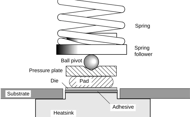
Flat sheets of rubber are frequently used to transfer a load from one planar surface to another. Such pads serve to reduce local pressure nonuniformities due to point defects (bumps and voids), as well as large scale distortions (warp, bow, waviness). But owing to the incompressibility of rubber, the pressure applied by a pad is not truly uniform, rather it tends to be highest at the center of the pad, decreasing toward the edges. In some microelectronic applications, such as when the pad contacts the active surface of a silicon microcircuit (die), this pressure nonuniformity is of tremendous importance. Rubber pad use in packaging can be temporary or permanent. An

Pad Substrate

Die

Heatsink Pressure plate

Spring

Ball pivot

Spring follower

[image:11.612.144.472.259.461.2]

Adhesive

Figure 1: High pressure adhesive die attach process.

example of temporary application occurs when a pad is used to load the adhesive joint during high pressure die attach as shown in Fig.1. The ball pivot keeps the spring force centered on the die, while the rubber pad distributes the force preventing excessive or spatially varying normal contact stresses which may cause die cracking or a nonuniform adhesive thickness distribution [1]. An example of permanent rubber pad application is depicted in Fig.2, where the pad is used in a package to press the die against a heatsink in order to form a pressure contact joint. A similar approach was used for a recent Siemens mainframe computer [2, 3]. In this case, contact stress gradients can lead to corresponding temperature gradients. Figure 2 also shows the importance of understanding pad deformation; if the edges of the pad bulge excessively, bondwire damage may occur. And in both cases, shear tractions applied to the active surface of the die may damage it.

Lid

Pad Substrate

Bondwires

Pressure Contact Joint Heatsink

Die

Figure 2: Pressure contact die attach with bondwires.

on the current study.

The force distribution could be modified by using a pad with a 3-D surface profile rather than a flat surface. To reduce costs and lead times, we chose instead to investigate the limitations of shapes stamped from flat stock with low cost punches and steel-rule dies. The Siemens mainframe is also reported to have used perforated pads [4].

We chose two elastomers for our investigation. The first was pure gum rubber, since it is one of the materials whose properties have been most widely reported in the open literature. The second was VitonTM _{[Du Pont], the fluoroelastomer we had already selected for our end}

use applications. Viton has excellent chemical resistance and tolerates high temperatures1 . And while it is much more expensive than conventional compounds, it is a fraction of the cost of fully fluorinated elastomers such as KalrezTM _{[Du Pont] and Chemraz}TM _{[Green, Tweed,}

& Co.]. Viton is also readily available in sheet form in both commercial and MIL-SPEC grades; this proved to be an important distinction. Viton is the commercial name of copolymers of vinylidene fluoride. Several types are available: Viton “A” is a dipolymer of vinylidene fluoride and hexafluoropropylene, Viton “B” and “F” are terpolymers of vinylidene fluoride and combinations of hexafluoropropylene and tetrafluoroethylene [5]. The main difference is their chemical resistance to aggressive substances. The elongation at break is rather low (about 200%) and these compounds are generally stiffer than other rubber-like materials [6].

The goal of our research was to develop a sufficient understanding of the behavior of small Viton pads, so that designers could quickly develop acceptable pressure pad designs without further detailed studies. Both numerical and experimental methods were used. Our work centered on optimizing the behavior a 14 mm square by 0.8 mm thick pad under a fixed normal force. Our primary optimization criteria was minimization of the maximum normal contact stresses applied by the pad surface.

1_{Viton has a long service life even with continuous exposure to 200}

2

Rubber Elasticity

2.1

Finite Elasticity

Rubber and rubber-like materials have the unique capability to withstand large deformations and still be able to fully recover their original dimensions. These materials owe their unusual properties to their molecular structure, which consists of long hydrocarbon chains (often with Cl or Fl substitutions) with a tangled shape and freely rotating links. The hydrocarbon molecules are interlocked in such a way that they form a three dimensional network able to sustain large deformations as chains straighten (Treloar [7] p.12.) Natural and syntehtic rubbers and their derivatives can achieve strains as high as 500%-1000%. In this case “strain” is defined as the percentage change in original length

L

,

"

=

∆

L

L

100 (1)

By contrast, most other engineering materials are only able to recover their initial dimensions for strains of at most a few tenths of a percent in uniaxial extension. Within those limits, both rubber and other solids behave elastically, which implies not only the recovery from any imposed deformations but also independence of stresses on previous deformation history.

Engineering materials such as crystalline metals are classified as linear elastic solids whereas

ε σ

Strain

Stress

ε ε

σ _σ

(a) Elastic (b) Nonlinear elastic (c) Inelastic

εb εa

[image:13.612.111.479.427.564.2]

unloading loading

Figure 3: Types of stress-strain responses

different paths. For a given strain, such as

"

b, there are two possible stress values depending on

previous loading history. Also, note that upon unloading to zero stress, the material has acquired a permanent deformation

"

a. This is called inelastic behavior, and is typical of materials when

the elastic limit is exceeded.

Deformations in metals loaded within the elastic limits are much less than unity and therefore their behavior can usually be adequately characterized with either a strength of materials approach or its more refined counterpart, the infinitesimal theory of elasticity. Rubber-like materials can exhibit strains that are several orders of magnitude higher, and the same approach cannot be used. The more general finite elasticity theory is needed. All measures, such as strains and stresses, defined for linear isotropic elastic solids have to be recast in the context of a finite deformation theory. It is noted that the infinitesimal theory constitutes a limiting case of the finite deformation theory. Only the fundamental concepts of finite elasticity will be presented here; the interested reader is referred to the many excellent treatises on continuum mechanics and nonlinear elasticity such as Malvern [8], Green and Adkins [9], and Green and Zerna [10].

One of the main differences between the infinitesimal and finite deformation theories is the location at which the stress and strain measures are defined. When deformations are large, the initial and final locations of a particular point such as P in Fig.30 (Appendix A, page 39) may be widely separated. In such cases, motions, strains, and stresses could be defined in two different ways, by referencing them to the initial undeformed configuration or to the current deformed configuration. These are the Lagrangian and Eulerian descriptions [8]. When deformations are small compared to unity, as with metals, this distinction becomes unnecessary and all stress and strain measures collapse into the definitions of the infinitesimal theory. The strain tensor, defined in the infinitesimal theory in terms of displacement gradients as

"

ij

=

1 2

@u

i

@x

j

+

@u

j

@x

i

!

(2)

where

"

ij : strains

u i,

u

j : displacements

is replaced in finite elasticity theory by either the Lagrangian or Eulerian finite strain tensor,

E

AB or

e

ij (see Appendix A, page 40 and ref.[8]).

Although it is possible to analyze rubber-like materials using finite strains, it is customary to instead use a stretch ratio,

, defined in the deformed configuration as the ratio of the original and current relative lengths (see Fig.30, page 39, and derivation in page 40),

1

=

dX

dx

(3)

The only differences are the values at zero deformation, where the stretch ratio is

=1 but the

indicates that the final dimension is twice the original one. The use of stretch ratios in finite elasticity is a matter of convenience due to the magnitude of the deformations. By contrast, using stretch ratios in the infinitesimal theory would be cumbersome at best. For example, an object with an original length of 1 mm and a final length of 1.001 mm, is much easier to describe using engineering strains (

"

=0

:

1%).

Stress measures in finite elasticity theory center around the Cauchy or true stresses which are defined in the deformed configuration2.

2.2

Stresses and Constitutive Equations

In most engineering design problems, the load acting on an object is known, or can be assumed to fall within in a certain range. Based on this, the analyst seeks to determine the corresponding effects in the interior of a solid, i.e., investigate stresses and their distribution. Stresses cannot be measured directly and must instead be related to measurable quantities such as strains or stretch ratios through the use of constitutive equations which describe the relationship between stresses and stretch ratios or strains. The independence of stresses on previous deformation history and the reversibility of imposed deformations in elastic materials allows us to prove that constitutive relations for both linear and nonlinear elastic solids can be derived from a strain energy potential function. This argument is very similar to the path independent work done on a particle in a potential field where the forces can be derived from a differentiable potential function [11]. By analogy, if stresses take the place of forces, a differentiable potential function must exist3_{that it is a function only of the deformations. In such cases stresses can be expressed}

as

ij

=

dW

(e)

de

ij

(4)

where

ij : true (Cauchy) stresses

W(e) : potential strain energy density function (strain energy per unit volume)

e : any deformation measure (e.g., finite Eulerian strain tensor, stretches)

Any material for which such a potential strain energy function exists is called a Green-elastic or hyperelastic material [8]. In the strictest terms, both linear and nonlinear elastic materials are hyperelastic. In practice however, the term hyperelastic is generally applied only to rubber-like materials. From the mathematical standpoint, there are two ways to apply Eq.4 to obtain a constitutive relation. One is to assume small strains, take a series expansion and consider only

2_{Stresses can also be referenced to the initial undeformed configuration (e.g. the first Piola-Kirchhoff stress}

tensor). This distinction is necessary due to changes in areas associated with the current and original configurations.

the linear terms. This leads to the familiar Hooke’s law for linear elastic solids. The other is to assume finite strains and construct a suitable strain energy function. The success of any analytical or numerical effort in hyperelastic solids depends closely on the ability of the chosen strain energy function to reproduce the actual material behavior.

In spite of their compliant appearance, most rubbers are incompressible or nearly incom-pressible solids. This makes them capable of withstanding large hydrostatic tractions without any change in volume and implies that deformations alone cannot describe stress states in the interior of such materials. For example, imagine a rubber ball deep in the ocean. It is subjected to homogeneous external tractions

p

=

gh

(

: water density,

g

: acceleration of gravity,

h

:

depth), yet due to its imcompressibility, it has the same dimensions as at sea level. This incom-pressibilty condition can be expressed as a function of the stretch ratios along three orthogonal directions,

1

2

3 =1 (5)

Our focus here will be on homogenous deformations, those in which the deformation gradient

F

i;A does not depend on the original configuration

X (see Appendix A, page 40). Such

deformations can be completely characterized with only three stretch ratios along orthogonal directions. The hydrostatic state of the ball in the ocean example is one case. Another is a sample subjected to biaxial extension along two orthogonal axes. Since the unit vectors associated with the original and deformed configurations (N andn) do not change orientation

in a homogeneous deformation, there is only one stretch measure (see Appendix A, page 41). In the general case of an isotropic hyperelastic solid, the strain energy density function

W

must be a symmetrical function of the stretch ratios

1,

2, and

3(see Rivlin [12] and Treloar

[7].) It follows that

W

can be defined in terms of the three invariants defined as (see Eq.52, Appendix A page 42),

I

1 =

2 1+

2 2+

2 3

I

2 =

2 1

2 2+

2 2

2 3+

2 1

2 3 (6)

I

3 =

2 1

2 2

2 3 Thus,

W

=

W

(

I

1

;I

2

;I

3) (7)

The choice of

W

can be arbitrary as long as it does not violate any of the principles of continuum mechanics (for example, it must predict zero stress at zero deformation). A suitable general form is a power series of the invariants

I

1,

I

2, and

I

3

W

(

I

1

;I

2

;I

3)=

1 X

i=0;j=0;k =0

C

ijk

(

I

1,3) i

(

I

2,3) j

(

I

3,1) k

(8)

C

ijk : material constants

This function is zero at zero deformation as long as

C

000=0. Also note that by Eq.6,

I

1=

I

2=3

and

I

3 =1 for

1 =

2 =

3 =1, and the correct zero stress is predicted by Eq.4.

When the incompressibility condition is introduced,

I

3 = 1 for any stress state, and the

terms affected by it drop from Eq.8 giving

W

(

I

1

;I

2)=

1 X

i=0;j=0

C

ij

(

I

1,3) i

(

I

2,3) j

(9)

where

C

ij : material constants

Again,

C

00=0 in order to have zero stresses at zero deformation. Generally the first few terms in

the series dominate, and we can consider

W

to be given by the two-term approximation which includes only the linear terms in

I

1and

I

2(

i

=1

;j

=0 and

i

=0

;j

=1),

W

(

I

1

;I

2)=

C

10(

I

1,3)+

C

01(

I

2,3) (10)

This is perhaps the form most widely used in rubber elasticity and is known as the Mooney-Rivlin strain energy function, first proposed by Mooney in 1940 [13, 12]. The Mooney-Mooney-Rivlin form has been found to reproduce the behavior of most natural and synthetic rubbers for moderate deformations (

4). For higher stretch ratios it is less successful, and over the

years, a number of other forms for the strain energy function have been proposed in response to the need to characterize a variety of rubber-like materials. Some of these are higher order approximations of Eq.9 and others have been formulated along rather different lines, among them:

Neo-Hookean form [7]

W

=

C

10(

I

1,3) (11)

Used only for certain vulcanized rubbers swollen with organic solvents [11]. It gives a poorer fit of experimental data than Mooney-Rivlin’s form.

Rivlin-Saunders form [14]

W

=

C

10(

I

1,3)+

F

(

I

2,3) (12)

where

F

(

I

2,3)is a function of

I

2. Intended for a general rubber-like material.

Klosner and Segal [15] cubic form for

F

(

I

2,3)

W

=

C

10(

I

1,3)+

C

01(

I

2,3)+

C

02(

I

2,3)

2

+

C

03(

I

2,3)

3

(13)

Ishihara et.al. form [16]

W

=

C

10(

I

1,3)+

C

20(

I

1,3)

2

+

C

01(

I

2,3) (14)

Obtained from non-Gaussian molecular theory considerations. It exhibits poor correlation with uniaxial experimental data on 8% sulfur rubber, Alexander [17].

Second order deformation form [37]

W

=

C

10(

I

1,3)+

C

01(

I

2,3)+

C

20(

I

1,3)

2

+

C

11(

I

1,3)(

I

2,3)+

C

02(

I

2,3)

2 ₍₁₅₎

General use. Included in some finite element programs.

Third order deformation form [18, 19]

W

=

C

10(

I

1,3)+

C

01(

I

2,3)+

C

20(

I

1,3)

2

+

C

11(

I

1,3)(

I

2,3)+

C

30(

I

1,3)

3 ₍₁₆₎

General use. Included in some finite element programs.

Yeoh form [20]

W

=

C

10(

I

1,3)+

C

20(

I

1,3)

2

+

C

30(

I

1,3)

3 ₍₁₇₎

Used for carbon black filled rubber vulcanizates in which material constants have a strain-history dependency. Of interest in the automotive tire industry.

Hart-Smith and Crisp [21, 22] exponential-hyperbolic form,

W

=

C

Z

e

k

1(I

1,3)

2

+

k

2

lnI

2

3

(18)

where

C

,

k

1, and

k

2 are material constants. Tested on sulfur rubber and cast latex. It

does not give good agreement in “Neoprene” (polychloroprene) film under equibiaxial stresses [17].

Alexander form [17]

W

=

C

1

Z

e

k (I1,3)

2

dI

1+

C

2

ln

I

2,3+

k

1

k

1

!

+

C

01(

I

2,3) (19)

Hutchinson, Becker, and Landel form [11]

W

=

C

10(

I

1,3)+

C

20(

I

1,3)

2

+

B

1(1,

e

k1(I2,3)

)+

B

2(1,

e

k2(I2,3)

) (20)

where

B

1,

B

2,

k

1, and

k

2are material constants. Good agreement for uniaxial and biaxial

tests on filled dimethyl siloxane (silicone) rubber.

Ogden form [23]

W

= 1 X i=1

i

i (

i 1 +

i 2 +

i

3 ,3) (21)

where

i,

iare material constants. Intended for general use.

The Ogden form, Eq.21, is a more general expression than the expansion in Eq.9. It redefines the first two invariants given by Eq.6 as

I

1 = (

1 1 +

1 2 +

1 3 ,3)

I

2 = (

2

1 +

2

2 +

2

3 ,3) (22)

where the exponents are not necessarily integers. When

1 = 2 and

2 = ,2, a two-term

Ogden formulation is identical to the Mooney-Rivlin strain energy function, Eq.10.

The choice of a strain energy function depends heavily on the material and the stretch ratios to which it will be subjected. For relatively small stretch ratios, say

<

2, a linear approximation such as Mooney-Rivlin’s is usually quite adequate, but for high stretch ratio ranges, a higher order approximation may be needed.

Once a strain energy function is chosen, one must still determine the material constants

C

ij,

i, etc., and the expression for the stresses. Considering stretch ratios as deformation measures,

the stresses are expressed using Eq.4,

ij

ij

=

i

@W

(

I

1

;I

2)

@

i

+

p

(23)

where

ij : Kroenecker delta

p : hydrostatic pressure

The additional term,

p

, can be considered a Lagrange multiplier needed to comply with the incompressibility condition and accounts for any hydrostatic tractions. For example, a uniaxial loading along the first axis can be described by the stretch ratios

1=

;

2 =

3 =

1

p

(since

1 is imposed,

2and

3 are considered to be equal and obtained from the

imcompress-ibility condition,

1

2

3 =1). If a Mooney-Rivlin material and zero hydrostatic tractions are

assumed, then the stresses from Eq.23 are

11=

@W

@I

1

@I

1

@

+

@W

@I

2

@I

2

@

! (24)

The invariants are (see Appendix A, page 42),

I

1 =

2 1+

2 2+

2 3 =

2 +2 1

I

2 =

1

2 1 + 1

2 2 + 1

2 3

=2

+

1

2

Substituting the derivatives of the invariants and the Mooney-Rivlin strain energy function into Eq.24 gives,

11=2

2

,

1

!

C

10+

1

C

01

!

(25)

Similar expresssions can be obtained for equibiaxial loadings

1=

2 =

;

3 =

1

2 (26)

11=

22 =2

2 , 1

4 !

C

10+

2

C

01

(27)

2.3

Application to Pad Design

Frictional forces on the interface

Rigid Plates

Rubber-like material

[image:21.612.129.468.109.261.2]

Compressive load

Figure 4: Effect of a finite friction coefficient on material confinement.

freely. This gives rise to substantial radial stress gradients. Placing a hole or perforation in the zone where confinement is expected allows the surrounding material to flow toward the hole’s free edge, relieving contact stresses in the vicinity. Our investigation was intended to explore the combined effects of hole placement and size on the contact stress distribution and to reduce its peak value.

In spite of their deceptively simple appearance, the closed form calculation of stresses from the analytical expressions presented so far can be made only in a limited number of cases with simple geometries, boundary conditions, and homogeneous deformations. Experimental methods can be used instead if the time and expense are justified. For example, the contact stress distribution in compressed rubber cylinders has been successfully analyzed by such a method [24]. However, in the vast majority of design cases where direct solutions are not possible the widespread availability of numerical methods such as nonlinear finite element analysis has reduced the need for experimental methods. Commercial codes that include several hyperelastic constitutive models are routinely used in the tire and automotive industries [19]. We chose the same approach to evaluate our pad designs. But first, we needed to determine the material constants for Viton.

3

Material Characterization

In order to use the constitutive models offered by finite element codes, it is necessary to provide values for the various material constants (

C

ij) defined in the previous section. Unfortunately,

least-squares fit of the data to an appropriate constitutive relationship. Since different loading modes have slightly different stress-stretch ratio responses, the test loading must be representative of the problem under consideration. It would be incorrect to use material constants obtained, say from an extension test, in a finite element model loaded under pure shear. If the primary loading mode is unknown, then several tests under different loading types are needed and the constitutive model fitted to all experimental points. 4

The most common homogeneous deformation tests are

Uniaxial extension

Equibiaxial extension

Pure shear

However, the primary loading mode of interest in the design of pressure pads is uniaxial compression. Curiously enough, the superposition principle can be used to show that uniaxial compression of a wide sheet (e.g. a pressure pad) is equivalent to uniform equibiaxial extension. To visualize this, consider the sheet in Fig.5(a), which is subjected to equibiaxial tractions

, and also subjected to a hydrostatic stress state,

. By the superposition principle, the hydrostatic

tractions at the edge of the sheet exactly cancel the tractions imposed by the equibiaxial extension. But the faces of the sheet are still subjected to the hydrostatic tractions. The net result is a sheet loaded in uniaxial compression. Hence, we choose an equibiaxial test as the

(a) biaxial extension + (b) hydrostatic compression = (c) uniaxial compression

σ _σ

−σ

−σ

[image:22.612.107.518.442.548.2]

−σ

Figure 5: Equivalency of uniform biaxial extension and uniaxial compression

primary means for obtaining material constants for Viton pressure pads.

There are several ways to obtain biaxial extension. One of them involves stretching a sheet of rubber in two orthogonal directions. However, there are a number of problems with this method: the difficulty of maintaining a constant 1:1 load ratio on the two loading directions and the clamping method. Clamping must usually be done with strings in order to avoid nonuniform transmission of the imposed load to the sheet. The load ratio problem can be solved by using

dead weights, springs, or a feedback control system with active loading devices. An additional problem is to maintain the load alignment with respect to the deforming sheet (remember the large deformations that rubber can attain). A detailed description of the experimental aspects of this method can be found in refs.[15, 25]5.

3.1

Inflation Test

An alternative biaxial extension method, the inflation test, is much simpler to implement. A circular sheet is clamped at its edge and subjected to internal pressurization. When inflated, the sheet acquires a balloon-like shape and as long as its radius of curvature is much greater than its thickness, it can be analyzed as a membrane . If only small areas are considered, say near the pole of the inflated shape, curvature effects can be safely ignored and the sheet can be considered to be under a uniform biaxial load. Historically, this was the first test used to characterize rubber behavior. Treloar and Rivlin and co-workers [26, 27, 28, 14] used it not only to find material constants but also to check the validity of a number of analytical solutions for the membrane inflation problem. Nowadays, the inflation test is used in almost all rubber-like material characterization cases related to numerical solutions and nonlinear finite element analysis [22, 29, 30]. It is also one of the most widely described tests for other applications such as mold filling problems [31]. The objective of an inflation test is to record the stretch ratios as a function of inflation pressure. The stretch ratio vs. pressure data is then processed to calculate material constants.

Three different materials were tested: natural latex, pure gum rubber, and Viton. The 0.8 mm (nominal) thick pure gum and natural latex sheets were used to gauge the validity of our methods by comparing results with published values. Mooney-Rivlin constants for pure gum rubber were previously obtained by Oden and Kubitza [29]. Our 0.8 mm nominal thickness Viton sheets were procured from three different sources6 _{in order to evaluate the variability}

of material constants. One source provided commercial grade sheets while two other vendors provided material conforming to MIL-R-83248 Type 2, class 1 specifications.

Sample preparation consisted of cutting circular sheets 81 mm in diameter from the un-deformed material7 and marking gage lines as indicated in Fig.6. Gage lengths of

l

0 = 6

mm were used for Viton and

l

0 =3 mm for natural latex and pure gum rubber. Longer gage

lengths were more appropriate for Viton samples due to their relatively low ultimate elongation values (approximately 150% per ASTM D 412 [32]). While other investigators recommended using the finest possible gage lines [14], we found this unnecessary since we were able to make

5_{The investigations reported in these references by Treloar and Klosner and Segal were concerned with biaxial}

loadings with ratios other than 1:1. Such biaxial tests are an alternative to a purely unixial test.

6_{See supplier list in App.B, page 44.}

7_{This did not correspond to the diameter of the free area able to deform during inflation, the free area is}

81mm

∅

l₀

Free area after clamping

35mm or 53.5mm

∅

[image:24.612.160.478.98.331.2]

Gage lines

Figure 6: Gage length tracing on a circular sheet

accurate measurements to the edges of the lines. A solvent-based metallic “silver marker” was found to give the best color contrast against the normally dark Viton. A 0.25mm drafting pen with water-based black ink was used to mark both the amber colored natural latex and light brown pure gum rubber. Ink adhesion proved to be very important, especially at large stretch ratios (

>

4) when lines tended to lose cohesion and “blur” due to the highly extended state of the material. An optical stage with an attached straight edge was used to accurately mark the gage lines. We also evaluated Nd:YAG laser marking, but found that visible marks damaged the material, particularly the heavily loaded Viton.

The apparatus used to perform the inflation tests consisted of a circular pressure chamber capped by the test sample and sealed with an annular clamp, Fig.7. Dry compressed air was used as the pressurizing fluid. The base and clamps were machined from 6061 aluminum stock. The base included ports for pressure measurements and to admit and vent air. Air inlet control was via a needle valve. Pressure measurements were made with a 0-344 kPa (0-50 psi) pressure transducer for Viton and a precision 0-206 kPa (0-30 psi) Bourdon gage for natural latex and pure gum rubber. Both instruments were calibrated against mercury and water manometers. Both pressure gages could be connected at the same time. A second needle valve was used to deflate the membrane while recording the corresponding stretch ratio response. The entire apparatus was designed to fit on the

x

,

y

stage of a Nikon universal measurement microscope.

Belleville spring washer

Clamp

Base Pressure

chamber

Air inlet Test sample

[image:25.612.165.463.89.484.2]

Pressure measurement Gage lines

Figure 7: Inflation test apparatus.

large radius of curvature in the inflated shape. Both clamps were machined with a beveled edge as depicted in Fig.7 to allow for free deformation of the inflated sheet. Belleville spring washers under the clamping bolts proved useful in preventing air leaks over the entire range of pressures. Insufficient clamping forces can allow slipping of the sheet between the clamp and base at high stretch ratios and be a source of experimental errors as noted by Hart-Smith and Crisp [22].

As the sample inflates, the original gage length

l

0 adopts a curved shape, so that direct

measurements of the stretched gage length

l

s are not possible. Instead, measurement of the

(

x;y;z

)coordinates of three points,

a

,

b

, and

c

, indicated in Fig.8 enables first computing the

a

b c

A B C

l =ABC₀ ls

Inflated shape

Undeformed shape

(x,y,z)_c (x,y,z)_b

(x,y,z)_a

x y

[image:26.612.134.495.100.340.2]

z

Figure 8: Inflated shape and deformed gage length.

pressure is then

=

l

s

l

0

(28)

It is not absolutely necessary that the deformed gage length be centered at the pole of the inflated shape. The location of point (

x;y;z

)

b in the neighborhood of the pole is enough to

ensure the validity of a biaxial stress state assumption. The ability to track the location of the deformed gage length

l

s is more important. The

(

x;y;z

)coordinates were determined by

translating the test apparatus under the microscope objective and focusing the crosshairs on the measurement point. The(

x;y

)values were obtained to1

m resolution from the digital

readout of linear encoders attached to the microscope stage. The extremely shallow depth of focus of the microscope allowed

z

-axis measurements repeatable to within0

:

5

m, as taken

from a second digital readout attached to the microscope objective’s rack. All three coordinate values were written simultaneously to a text file through an RS-232 interface. Pressure values were recorded manually when using the 0-206 kPa (0-30 psi.) Bourdon gage and written to a separate text file when employing the 0-344 kPa (0-50 psi.) pressure transducer. The test procedure is summarized below:

1 - Measure original gage length.

2 - Admit air.

4 - Measure pressure.

5 - Repeat steps 2-4 until the preset maximum pressure.

6 - Vent air in steps and repeat measurement to assess hysteresis.

Viton exhibited a noticeable viscoelastic behavior, which complicated testing. Upon a step pressurization, the membrane would not immediately assume an equilibrium position. Before making a measurement, it was necessary to wait between 5 and 30 min. depending on the stretch ratios.

At high pressures, the gage lines tended to blur due to the separation of the ink particles. This made it difficult to locate measurement points through the microscope. In the case of natural latex, the line blurring problem was exacerbated by membrane thinning at high stretch ratios. By Eq.26, the thickness

t

sof the latex membrane subjected to the maximum stretch ratio

1 =

2 =

=4

:

86 achieved during the test is

t

s

=

t

0

2 =

1 23

:

6

t

0

=32

:

2

m

(29)

(

3 =

t

s

=t

0 where

t

0

=0.762 mm was the original undeformed thickness). At this thickness

natural latex becomes almost translucent, reducing the contrast of the gage lines. Changing the microscope magnification from 20to 5, and reducing lighting helped to mitigate the

problem.

One of the peculiarities of rubber-like materials is the nonmonotonic form of the measured inflation pressure vs. stretch ratio curve, shown in Fig.9 for natural latex. At a certain value

2 3 4 10

20 30 40

5 1

Inflation pressure p [kPa]

λ

Deflation

Inflation

Natural latex

: 35 mm

∅

[image:27.612.140.458.463.652.2]

0.762 mm t :₀

Figure 9: Measured inflation pressure vs. stretch ratio curve for natural latex.

1.2 1.4 1.6 1.8 2.2 2.4 2.6 100

150 200

2.0 1.0

50 250

Inflation pressure p [kPa]

λ

Viton™

: 53.5 mm

∅

0.863 mm t :₀

Inflation

Last recorded point before bursting

[image:28.612.139.449.94.285.2]

Supplier: McMaster-Carr

Figure 10: Measured inflation pressure vs. stretch ratio curve for Viton.

raising the internal pressure8_{. As still more air is added, the internal pressure stabilizes and}

then starts increasing again, indicating less compliance to deformations. This apparent strain hardening is attributed to crystalization phenomena in rubber-like materials [33]. As shown in Fig.10, Viton did not exhibit pressure stabilization, rather it burst shortly after a slight drop in inflation pressure. The non-monotonicity of the inflation pressure represents an unstable bifurcation behavior9since more than one stretch ratio is possible for a given inflation pressure [11, 29]. This problem was extensively studied due to its influence on flight prediction of meteorological balloons, Alexander [33] and Needleman [34]. A leak-free test assembly has proven necessary in order to accurately discern the onset of this phenomenon.

3.2

Data Reduction and Calculation of Material Constants

The inflation test yields a series of measurements of grid line mark positions vs. inflation pressure. This data is reduced by the following steps to yield true membrane stress vs. stretch ratios:

1 - convert coordinate measurements to radii of curvature.

2 - calculate of deformed gage lengths using radii of curvature and(

x;y;z

)coordinates.

3 - calculate stretch ratios.

4 - calculate the biaxial true (Cauchy) stresses in the neighborhood of the measurement points.

8_{This phenomenon is familiar to anyone who has ever tried to inflate a balloon. It is difficult to get the balloon}

started, but once it reaches a certain size it fills the rest of the way more easily.

Assuming that the original and deformed gage lengths are coplanar, the radius of curvature

r

of the curvea,b,c(Fig.11) can be obtained by trigonometric relations as

r

2

=

1 4

(∆

x

2 1+∆

z

2 1)(∆

x

2 2+∆

z

2

2)[(∆

x

1+∆

x

2)

2

+(∆

z

1,∆

z

2)

2

]

(∆

x

1∆

z

2+∆

z

1∆

x

2)

2 (30)

where all quantities are defined in Fig.11. This was the approach used by Rivlin and Saunders

a

b

c

x

a xb xc

l_s

z

a

z_c z

b

x = x - x_{1 b a} x = x - x_{2 c b}

z = z - z_{1 b a} z = z - z_{2 b c}

x x

r

θ

[image:29.612.130.504.213.475.2]

Deformed gage length

Figure 11: Computation of deformed gage lengths from coordinate measurements.

[14]10. The angle

subtended by the deformed gage length

l

sis

=2

sin

,1 1

2

r

q

(∆

x

1+∆

x

2)

2

+(∆

z

1,∆

z

2)

2 ₍₃₁₎

Since

r >> l

sthe deformed length

l

scan be found as

l

s

=

r

(32)

And by Eq.28, the stretch ratio is

=

l

s

l

0

10_{An alternative expression can be derived using shell theory and by assuming a nearly spherical inflated shape}

The true stresses in the neighborhood of the pole of the inflated shape can be found from the well-known expression for the stresses in a membrane under uniform pressure,

=

11=

22 =

pr

2

t

s

(33)

where

11,22: stresses

p : inflation pressure

r : radius of curvature

t

s : thickness in the deformed state

Except for

t

s, all quantities on the right hand side of this expression can be measured or

computed. By Eq.29,

t

sis a function of the original thickness and the stretch ratio. The stresses

are then

11=

22 =

pr

2

t

0

2

(34)

At this point, the experimental data have been converted into pairs of

vs.

values. A sample plot obtained for pure gum rubber is shown in Fig.12. The next step is to choose a strain energy function and determine the material constants.

1.5 2 2.5 3 3.5 4 4.5 2.5

5.0 7.5 10 12.5 15

λ σ

Membrane Stresses [MPa]

1

Pure Gum rubber

: 35 mm

∅

[image:30.612.148.441.389.583.2]

0.787 mm t :₀

Figure 12: Experimental data points,

vs.

for pure gum rubber

to calculate the coefficients that minimize the error in fitting the experimental data points such as those indicated in Fig.12. In this case, instead of choosing any function, the analytical expression for the stresses according to Eq.27 is taken as the interpolating function.

ˆ

f

(

j

)=2

2 j , 1

4 j !

C

10+2

4 j , 1

2 j !

C

01 =

j (35)

where

ˆ

f( j

) : interpolating function

j :

jth true stress from the experimental data

j : corresponding stretch ratio

The unknowns are the Mooney-Rivlin constants

C

10and

C

01. Note that Eq.35 is linear in

C

10

and

C

01, which allows the use of a linear least squares procedure (by contrast, Ogden’s strain

energy function, Eq.21, is nonlinear in the material constants

iand requires a nonlinear least

squares procedure, Twizell and Ogden [35].) The goal is to minimize the following function (see for example, ref.[36] p.258),

F

(

C

10

;C

01)=

n X

j=1

[

C

10

'

1(

j

)+

C

01

'

2(

j ),

j ] 2 ₍₃₆₎ where

n : number of experimental data points

and

'

1(

j

) = 2

2 j , 1

4 j !

'

2(

j

) = 2

4 j , 1

2 j !

The points

j that comply with Eq.36 must satisfy the conditions

@F

(

C

10

;C

01)

@C

10

=0

@F

(

C

10

;C

01)

@C

01 =0 i.e., 2 n X j=1

[

C

10

'

1(

j

)+

C

01

'

2(

j

),

j

]

'

1(

j

)=0

2

n X

j=1

[

C

10

'

1(

j

)+

C

01

'

2(

j

),

j

]

'

2(

j

which can be arranged as a system of two linear equations from which

C

10 and

C

01 can be readily obtained, 8 > > > > > > < > > > > > > : 2 4 n X j=1

'

2 1(

j ) 3 5

C

10+ 2 4 n X j=1

'

1(

j )

'

2(

j ) 3 5

C

01 = n X j=1

'

1(

j )

j 2 4 n X j=1

'

1(

j )

'

2(

j ) 3 5

C

10+ 2 4 n X j=1

'

2 2(

j ) 3 5

C

01 = n X j=1

'

2(

j )

j

(37)

An example of this calculation for pure gum rubber can be found in Appendix B, page 46; the results are plotted in Fig.13 with the fitting function superposed on the experimental data points. Table 1 compares the resulting material constants with those obtained by Oden and

1.5 2 2.5 3 3.5 4 4.5 2.5 5.0 7.5 10 12.5 15 σ

Membrane Stresses [MPa]

1

Linear least squares fit Experimental

C = 134.36 kPa C = 12.49 kPa10₀₁ Pure Gum rubber

λ

: 35 mm

∅

[image:32.612.165.448.284.468.2]

0.787 mm t :₀

Figure 13: Example of least squares fit of the Mooney-Rivlin form to experimental data.

[image:32.612.153.459.568.684.2]

Kubitza [29] for a similar material. The results are in reasonable agreement in spite of the fact the tests were performed with markedly different specimen sizes.

Table 1

Mooney-Rivlin Constants for Pure Gum Rubber

C

10

C

01

Present results 134.36 kPa 12.49 kPa

(D=35mm,t0=0.78mm) (1.37 kg/cm

2_{) (0.127 kg/cm}2₎

Oden-Kubitza[29] 111.79 kPa 13.73 kPa

(D=381mm,t0=1.78mm) (1.14 kg/cm

2_{) (0.14 kg/cm}2₎

[image:33.612.153.462.97.215.2]

Table 2

Mooney-Rivlin Constants for VitonTM

Supplier (dimensions)

C

10

C

01

McMaster-Carr 1194.6 kPa 163.0 kPa

(D=53.5mmt0=0.863mm) (12.18 kg/cm

2_{) (1.66 kg/cm}2₎

West American Rubber 1329.2 kPa 263.0 kPa

(D=53.5mmt0=0.838mm) (13.55 kg/cm

2_{) (2.69 kg/cm}2₎

D: diameter free to inflate,t0: initial thickness

NOTE: MIL-R-83248 Type 2, class 1 material specifications

Table 2 shows the material constants for MIL-SPEC grade Viton test samples obtained from two different vendors. These values turned out to be considerably higher than the constants for pure gum rubber. A third commercial-grade Viton sample was not tested due to its extremely low elongation at break (estimated at less than 130%) and its chemical susceptibility to the solvent-based marker used to trace the gage lines.

The values for

C

10 and

C

01 listed for the first sample of Viton were checked with a simple

four-element finite element model of a flat sheet intended to simulate the zone near the pole of

1.2 1.4 1.6 1.8 2.2 2.4 2.6 5

10 15 20 25 30

2.0 FE modeling

Inflation test

σ

[MPa]

λ

Viton™

1.0

[image:33.612.137.478.406.578.2]

Supplier: McMaster-Carr

Figure 14: Comparison of experimental data with a finite element model.

these constants are assumed to be valid as long as the deformation remains “as homogeneous as possible.”

4

Finite Element Modeling of the Proposed Shapes

A commercial finite element modeling program, Abaqus v.5-2 [37], was chosen to qualify our experimental results and to evaluate proposed pad designs. Abaqus includes strain energy functions valid for several hyperelastic constitutive models:

Mooney-Rivlin’s form (Eq.10)

Second order deformation form (Eq.15)

Ogden’s form (Eq.21)

It also includes the Neo-Hookean form since it can be obtained as a particular case of the Mooney-Rivlin form with

C

01 = 0. Ogden’s strain energy function can be formulated with

up to a six term (n=6) approximation of Eq.21. In addition, any of the constitutive models presented previously can be included through a user-defined subroutine (UHYPER).

A Digital Equipment Corporation Alpha AXP-based workstation was used to run all finite element models. Typical CPU times ranged from a few minutes to several hours depending on the loading level and degree of mesh refinement. With the exception of a few simple models, Patran v.3 [38] was used for mesh generation.

4.1

Model Description

The pressure pad problem was modeled with the following assumptions,

1 - Perfect adhesion of the pad faces to the compressing surfaces (once in contact, the pad faces do not separate). This assumption is usually valid for the high pressure die attach process where one side the pad is held by the rough active surface of the die and the other side is glued to the pressure plate (see Fig.1).

2 - Constant load applied by the compressing surfaces (as opposed to constant normal trac-tions).

A typical mesh used to model a square pad with a central hole will be used as an example to describe the finite element modeling. A three-dimensional model was adopted since the objective was to study contact stresses and visualize their distribution on the pad faces. Due to the symmetry of the geometry, boundary conditions, and loads, the modeling can be done on one eighth of the actual square pad. The effect of the rest of the pad can be modeled by imposing the appropriate boundary conditions to the model as indicated in Fig.15. The midsurface nodes are constrained to remain on the same

x

,

y

plane at all times during the loading history (when

u

z displacements occur, these nodes move as a whole, but independent movements in the

x

and

y

directions are still possible). Again, by symmetry considerations only one of the rigid compressing surfaces is modeled.

Three-dimensional eight-node linear-interpolation mixed-formulation elements were used

x y

z

1 model 8

u =0_y u =0_x

the same for all nodes at model upper surface (corresponds to pad’s midsurface)

u_z

Pad

Rigid surface

Full model

l/2 l

[image:35.612.111.504.287.618.2]

t/2 t

Figure 15: Pressure pad modeling and boundary conditons.

rubber-like materials for which the stresses cannot be uniquely determined from the displacements11_.

Three hundred and ninety 3-D elements were defined for the example in Fig.16. Only three elements were used along the thickness to maintain an adequate aspect ratio in the entire model. The height of all elements were the same, but an alternative “pre-distorted” mesh for extremely high loads may consider unequal element heights. Such a mesh is generated in a way that “negates” unfavorable distortions under loads, by making the original element shapes as if they were deformed in the opposite direction.

x y

z

C3D8H 3-D elements

C3D6H triangular prism elements (mesh fillers)

2.4 x 10 m-3

7 x 10 m-3

P

0

Figure 16: Mesh modeling a pad with a central hole.

A different type of element was used to model the interaction of the lower pad face with the rigid compressing surface. The three dimensionalC3D8Helements in the mesh of Fig.17 were overlaid on the lower surface with interface elementsIRS4capable of detecting contact with a separately defined rigid surface. The lateral edges were also covered with interface elements to model possible bulging and contact with the rigid surface. However, only two rows of lateral interface elements were defined. TheC3D8Helements adjacent to the midsurface of the actual pad (upper surface of the model) did not include them due to the kinematic constraint defined on its constituent nodes (they always remain in the same

x

,

y

plane). If interface elements

were defined there, the contact force would become undetermined if actual contact occured. Fortunately, extreme lateral bulging was not expected to occur with the loads of the case under study (if it were, the problem could be solved by defining more elements along the thickness). Interface elements also have the ability to deform with the 3-D elements to which they are attached and thus give the true (Cauchy) contact stresses on the rigid surface. The plots shown in the next subsection that describe the distribution of contact stresses are actually describing

11_{Traditional displacement-based elements have only displacements as field variables and calculate stresses}

IRS4 “interface” elements C3D8H elements

x y

z

[image:37.612.170.416.102.364.2]

Lateral interface elements

Figure 17: Use of interface elements to detect contact stresses.

tractions applied by the rubber pad to the interface elements. Friction between the interface elements and the rigid surface was considered to be infinite (perfect adhesion) but could have been modeled with any values from 0 to1.

A concentrated constant load

P

was applied in the ,

z

direction to the upper surface of

the mesh (midsurface of the actual pad), Fig.16. This load was automatically considered by Abaqus as uniformly distributed over the entire upper surface due to the kinematic constraint of its nodes (which are prescribed to remain in the same

x

,

y

plane).

The model depicted in Fig.16 consists of 610 nodes and 592 elements including the interface elements and has anRMSwavefront of 395 after internal optimization performed by Abaqus. The input file corresponding to this example is included in Appendix C, page 47.

4.2

Finite Element Modeling Results

Due to the kinematic constraints imposed by a large friction coefficient, the contact stresses originated by the compression of a solid rubber pad against a rigid surface are nonuniform, as shown in Fig.18(a). This plot was obtained by modeling one eighth of a 1414 square by

decrease toward the edges reaching a value of 71.3 kPa at the corners12_{. The distribution of}

contact shear stresses in the x-axis direction is also nonuniform as shown in Fig.18(b). In this case there is a sign reversal, with a peak contact shear stress of +85.6 kPa at the right edge and a minimum of -207 kPa along the vertical axis. Note that there are also contact shear

0

628 kPa

314

816

-207

-94.5

+18

+85.6 kPa

y

x y

x

xx

+σ

xx

−σ

(a) (b)

Figure 18: Normal (a) and shear (b) contact stresses applied by a 14140.8mm solid Viton

pad. One-eighth finite element model with a 19.6 N normal load (uniform compressive tractions of 400kPa).

0

100

250

375

500

650 kPa

Figure 19: Distribution of normal contact stresses in a 14140.8mm perforated pad. Hole

diameter: 1.2mm. One-eighth finite element model with a 19.6 N normal load.

stresses in the y-axis direction, whose distribution is the mirror image of Fig.18(b). Therefore, the true peak values differ from these values and must be found pointwise by performing the

12_{The contact stresses reported here follow Abaqus’ sign convention in which tractions and stresses are positive}

corresponding transformation. An upper bound on the true peak value is

p

2 times the maximum contact shear stress along a given axis. The signs refer to the direction of the contact shear stresses, positive along the +x direction and negative otherwise. At this load, the amount of lateral bulging at the midsurface of the pad is minimal (7

:

610

,

3 mm). The mesh used to model the solid pad is shown in Fig.20. It models one-eighth of the pad and consists of 162 three-dimensionalC3D8Helements and 99IRS4interface elements. The normal load applied to the upper surface of the model (midsurface of the actual pad) was 19.6 N, which is equivalent to 400 kPa when distributed over the entire model’s surface.

As noted on page 11, the introduction of a small through hole in the pad relieves the normal contact stresses in its vicinity since the surrounding material is able to deform with relative freedom. If only one hole is placed in the center of the pad while maintaining the same normal load and pad dimensions, the distribution of normal contact stress changes as shown in Fig.19. With a hole of 1.2mm in diameter, the region of peak stresses shifts to a roughly annular zone

P

x y

z

7 x 10 m-3 7 x 10 m-3

Figure 20: Mesh modeling a solid square pad.

surrounding the central hole and the maximum value drops 20% to 650 kPa. Note that the normal load applied to the finite element model was the same used for the solid square pad (19.6N) which implies that the average stress is higher than the previous case due to the loss of cross sectional area at the hole. By contrast, the peak values for contact shear stresses increase to +104 kPa and -606 kPa. The finite element model used for this case is similar to the one described in section 4.1. The hole diameter can be increased with a slight reduction of the peak normal contact stress but eventually it begins to increase again due to the effect of the reduced cross sectional area.

4 mm

∅1.2 mm

14 mm

[image:40.612.142.483.332.667.2]

Thickness 0.8mm

Figure 21: Pad perforated with a symmetrical array of four holes.

Location

(x,y) mm 1.2mm 2.4mm 4.8mm

(3.5,3.5)

(2.6,2.6)

(2,2)

(0,0) 1

4

4

4 # holes

Hole Diameter

0

993 kPa 1160 1780

831 779 893

589 667

650 638 682

816

-217 +216 -251 +241 -340 +398 -427 +216

-335 +182

-606 +104 -317 +116 -212 +151 -218 +177

-207 +85

-370 +223 -328 +349

Peak normal contact stress Max. and Min. shear contact stress [kPa]

No hole

( )σ_xx y

x

( )σ_zz

0

993

Hole center at (3.5,3.5) mm

Hole 1.2 mm∅ ∅ 2.4 mm ∅ 4.8 mm

0 0

y

x

382

764

kPa kPa _kPa

1160

899

449 688

1370

1780

0 0 0

(2.6,2.6)

319

689

831

299

599

779

343

687

893

0

256

(2,2)

226

453

589

0

513

667

0 0 0

(0,0)

250

500

650

245

491

638

262

524

682

0

No hole

314

628

[image:41.612.75.534.85.691.2]

816

-217 -251 -340

kPa kPa _kPa

-50

+116

+216

-61

+128

+241 +398

+227

-56

(3.5,3.5)

Hole 1.2 mm∅ ∅ 2.4 mm ∅ 4.8 mm

y

x

-427 -370 -328

-179

+67

+216 +223

+86

-142

+349

+193

-67

(2.6,2.6)

-335 -218

-136

+63

+182 +177

+86

-66

(2,2)

-606 -317 -212

-333

+59

+104 +116

+16

-150

+151

+67

-72

(0,0)

-207

-94

+18

+85

No hole

xx

+σ

Shear stress signs

xx

[image:42.612.75.535.85.686.2]

−σ

For a symmetrical four-hole array, the placement as well as the diameters of holes can be changed. Peak normal and shear contact stresses for all cases are summarized in Fig.22. Complete plots for normal and shear contact stresses are shown in Figs.23-24. It is noted that no attempt has been made to consider viscoelastic effects in the finite element modeling. Therefore, the long term values of the peak contact stresses are predicted to fall from the values listed in Fig.22 when a viscoelastic constitutive model is included. However, the stress values predicted without considering viscoelasticity are still valid as upper bounds in any given design.

5

Experimental Verification

To verify our finite element modeling of Viton pad deformation and contact stress distribution, and to investigate the effect of interfacial friction, we built a pad test apparatus that allowed

Viewport

Short stroke air cylinder Load

cell Optical flat

x,y

measurement stage

Test sample

Ball pivot Pressure _plate Signal

Air supply

[image:43.612.114.451.297.655.2]

Load cell shaft

Figure 25: Pad test apparatus.