HUNTING SEARCH ALGORITHM TO SOLVE THE
TRAVELING SALESMAN PROBLEM
1
AMINE AGHARGHOR, 2MOHAMMED ESSAID RIFFI
1Research Scholar, Department of Computer Science, Laboratory of LAROSERI, Faculty of Sciences,
Chouaïb Doukkali University, El Jadida, Morocco
2Professor, Department of Computer Science, Laboratory of LAROSERI, Faculty of Sciences, Chouaïb
Doukkali University, El Jadida, Morocco E-mail: [email protected], [email protected]
ABSTRACT
Traveling salesman problem is a classic combinatorial optimization problem NP-hard. It is often used to evaluate the performance of new optimization methods. We propose in the present article to evaluate the performance of the new Hunting Search method to find better results for the traveling salesman problem. Hunting Search is a meta-heuristic inspired by the method of group hunting of predatory animals. It is part of the evolutionary algorithms used to solve the continuation optimization problems. The work presents an adaptation of this method in a discrete case by redefining operations of the method into operations of permutation in the path of the visited cities of the traveling salesman. The proposed method was tested on the instances of reference of TSPLib Library and it gave good results compared to the recent optimization methods.
Keywords: Hunting Search; Traveling Salesman Problem; Combinatorial Optimization; Meta-heuristic;
1. INTRODUCTION
Traveling salesman problem (TSP) [1] is to find the shortest path to visit a given number of cities. The traveler just goes to each city once and returns to the city of departure. TSP is a combinatorial optimization problem of NP-hard class whose computational complexity increases exponentially by increasing the number of cities. The importance of this problem appears in many application areas such as transportation [2] and logistics [3]. Several combinatorial optimization problems in various fields are modeled as TSP such as the problem of Vehicle Routing [4] and the problem of Optimal Foraging [5]. In order to solve the TSP, several methods have been proposed: exact methods such as Branch-and-Bound algorithm [6], Cutting-Plane [7] and Brunch-Cut method [8]. Approximate methods such as Lin-Kernighan (LK) [9], Local Search [10], Descent [11], Tabou Search (TS) [12], Genetic Algorithm (GA) [13], Simulated Annealing (SA) [14], Ant Colony Algorithm (ACO) [15, 16], Bee Colony Optimization (BCO) [17], Particle Swarm Optimization (PSO) [18] and Harmony Search (HS) [19]. Exact methods are efficient only for the TSP small instances as it gives an exact optimum in a long duration. Approximate methods are used to solve TSP instances of all sizes as it
gives an approximate optimum in a short duration compared to exact methods. Researchers are still looking for methods that are more effective; that is why we propose the Hunting Search method for solving TSP.
Hunting Search (HuS) is an approximate continuous optimization method proposed by R. Oftadeh et al [20]. It is a meta-heuristic method inspired by group hunting of some animals such as wolves and lions. They are hunters who organize their position to surround the prey; each of them is relative to the position of others and especially in relation to the position of their leaders.
This paper proposes the use of the new powerful HuS method for solving a combinatorial optimization problem; the TSP, to find better optimized results. This adaptation to the discrete case is done by redefining the signification of each HuS parameter, searching the best parameters values and redefining the HuS operators.
instances of TSPLib Library are presented in the
fifth section and the last section is the conclusion of the whole work.
2. TRAVELING SALESMAN PROBLEM
TSP is a combinatorial optimization problem (or discrete optimization) where the best solution is defined by an objective function of a subset of a feasible solution from discrete set of feasible solutions.
Let E be the set of discrete feasible solutions, S is the subset of the feasible solutions of
E, ∶ → is the objective function. The problem is to find:
∶ ∈
E is the set of feasible Hamiltonian cycles,
S is the set of Hamiltonian cycles measured by the objective function. The objective function gives the distance of a Hamiltonian cycle defined as follows:
, !" #$ , %
Such as ∈ , vertices of , number of vertices of and & , '( is the distance between and '.
3. HUNTING SEARCH METHOD
HuS is an algorithm for solving continuous optimization problems. It is a meta-heuristic that uses the techniques of group hunting of some animals such as dolphins. The hunting group is represented by a set of solutions where each hunter is represented by one of these solutions. The leader of the hunting is the best solution. A hunter is characterized by its position that defines the distance between him and the other hunters.
During the hunt, hunters change their positions to better encircle their prey by movements toward their leader or by correcting their position relative to each other. Finally, if they are very close to each other or stuck, they have to be reorganized.
HuS is an evolutionary algorithm since it evolves a population of individuals (hunters) via operator selection and variation, in a manner similar to the evolution of living beings.
HuS algorithm is as follows: Initialize the parameters
Initialize the Hunting Group (HG)
Make a loop of NE iterations
Make a loop of IE iterations
Move toward the leader Correct the positions
If the distance between the best
and the worst hunter<EPS
Leave the loop iterations
of IE to the reorganization
End if
End loop iterations of IE
Reorganization hunters
End loop iteration of NE
4. ADAPTING HUNTING SEARCH TO THE
TRAVELING SALESMAN PROBLEM 4.1 Initialize the Hunting Group
It represents the group of hunters (set of the initial solution) by a two-dimensional array HG
of NC columns and HGS rows. It can also be represented as a matrix HG=(h1, h2, …, hHGS) of content (numbers and positions of the cities to be visited by the traveling salesman) randomly generated by the computer from a map of cities. Each row of the matrix will represent a solution to the problem. The distance traveled by the traveling salesman in each solution is calculated by the objective function (2) and define the best solution.
Where
NC (Number of Cities) is the number of cities to be visited by the traveling salesman.
HGS (Hunting Group Size) is the number of manipulated solutions.
Example contents of a table cell City number: 5
Figure 1: Illustration of the general form of a set of solutions
4.2 Move Toward the Leader
The new matrix HG’=(h1’, h2’, …, h’HGS) is built by a movement of the hunters toward the leader as follows:
hi’ = hi + rand x MML x (hL – hi) (3)
Where
MML (Maximum Movement toward the Leader) is a number between 0 and 1 representing closer rate of a hunter to the leader.
Rand is a uniform random number that varies between 0 and 1.
hL is the leader.
(hL – hi) refers to the distance between the best and the ith hunter. In this problem (TSP), the distance between two solutions is the number of cells of the two arrays that represents the two solutions that don’t have the same content (the same cities).
The operation '+' means copying a part of a solution in another one. Here, we talk about copying a part of the solution representing the hunter hL in the solution representing the hunter hi, rand×MML×(hL-hi) is the size of the part of the hunter hL to put in the hunter hi. For example, if rand=0.6, MML=0.3 and (hL – hi)=22; the size of
the part to be taken is four cells. Figure 2 is an example of copying a part of three cells from the hunter hL in hunter h1.
h1 5 3 2 1 6 4
h2 1 2 3 5 4 6
hL 2 6 5 4 3 1
h4 6 5 3 4 1 2
h1 2 6 5 4 3 1
h2 1 2 3 5 4 6
hL 2 6 5 4 3 1
h4 6 5 3 4 1 2
Figure 2: A hunter moving toward the leader
A new hunter is valid only if it is better than the old one, otherwise, we keep the old.
4.3 Correct the Positions
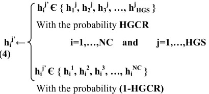
This is the stage where the hunters change their position relative to each other,the new group of hunters HG’=(h1’,h2’, …, h’HGS), which for every hunter hi, we have hi=(hi1, hi2, …, hiNC) is built through exchanges between these hunters of some parts of their solution as follows:
hi j’
Є { h1 j
, h2 j
, h3 j
, …, hjHGS }
With the probability HGCR
hi j’
← i=1,…,NC and j=1,…,HGS
(4)
hi j’
Є { hi 1
, hi 2
, hi 3
, …, hi NC
}
With the probability (1-HGCR)
Where
HGCR (Hunting Group Consideration Rate) is a number between 0 and 1 which represents the probability that a hunter makes a move to another hunter as copying a part of the solution representing the first one in the solution representing the second as described in (4) in the case of HGCR. Figure 3 is an example of copying a part of two cells from the hunter h3 into the hunter h1.
h
1,1h
1,2h
1,3…
h
1,NCh
2,1h
2,2h
2,3…
h
2,NCh
3,1h
3,2h
3,3…
h
3,NC…
…
…
…
…
[image:3.595.306.511.484.576.2]h1 5 3 2 1 6 4
h2 1 2 3 5 4 6
h3 2 6 5 4 3 1
h4 6 5 3 4 1 2
h1 2 3 5 4 6 1
h2 1 2 3 5 4 6
h3 2 6 5 4 3 1
[image:4.595.93.274.108.327.2]h4 6 5 3 4 1 2
Figure 3: Position correction of the hunter h1 relative to hunter h3 in the case of HGSR
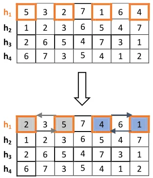
(1-HGCR) is the probability that a hunter changes its position with a permutation of k cells (k>=2) from its solution in a random manner as described in (4). Figure 4 is an example of swapping four cells from hunter h1.
h1 5 3 2 7 1 6 4
h2 1 2 3 6 5 4 7
h3 2 6 5 4 7 3 1
h4 6 7 3 5 4 1 2
h1 2 3 5 7 4 6 1
h2 1 2 3 6 5 4 7
h3 2 6 5 4 7 3 1
[image:4.595.114.271.433.615.2]h4 6 7 3 5 4 1 2
Figure 4: Position correction of the hunter h1 in the
case of (1-HGCR)
4.4 Reorganization hunters
During the process of the hunt, hunters may get blocked in a position (local solution) as they can’t have their prey. If this is the case, we made a reorganization to have another opportunity to find the best position (final solution).
The reorganization is the creation of a new group of hunters of random values from the old one. This new group of hunters replaces the old group, but preserves the previous best hunter.
We made reorganization in two cases:
• When the difference between the distance traveled by the leader and the worst hunter is less than EPS.
• When we end an epoch (when the IE
loop iterations are finished).
Where
NE (Number of Epochs) is the number of times to run the IE loop during the search.
IE (Iteration per Epoch) is the number of times to move toward leader and correct the hunters’ position.
EPS (Epsilon) is the minimum distance between the leader and the worst hunter.
5. EXPERIMENTAL RESULTS
This section presents performance tests of HuS algorithm on Euclidean instances of TSPLIB Library [21]. The tests were performed on a computer processor Intel (R) Core (TM) i5-2450M CPU 2.50GHz @ 2.50 GHz and 4 GB of RAM. The adaptation of the proposed algorithm is coded into a program language C# on visual studio 2012. 10 times tested for each instance.
Table 1 shows the HuS parameter values used in the tests.
Table1: Parameters Values
Parameters Values
Hunting group size
(HGS) 100
Maximum movement
toward leader (MML) 0.4
Hunting group consideration rate
(HGSR)
0.4
Maximum number of
epochs (NE) 10
Iteration per epoch
(IE) 50
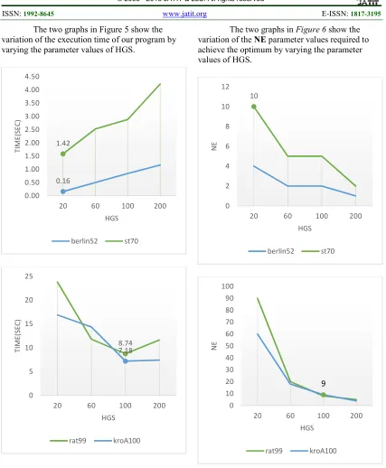
The two graphs in Figure 5 show the [image:5.595.86.513.100.618.2]
variation of the execution time of our program by varying the parameter values of HGS.
Figure 5: Run time obtained by varying HGS parameter value
We can see that for instances of size less than 99, the best value is HGS=20. For instances of size greater than or equal to 99, the best value is
HGS=100.
The two graphs in Figure 6 show the variation of the NE parameter values required to achieve the optimum by varying the parameter values of HGS.
Figure 6: NE obtained by varying HGS parameter value
According to the graphs, we can see that increasing the size of the HGS lowers NE. We can also see that the maximum number of epoch needed to achieve the optimum for HGS=20 and HGS=100 is NE=10.
The two graphs in Figure 7 show the variation of the percentage of TN compared to EN
by varying the parameters values of MML and IE.
TN (Number of times Trapped) is the number of
0.16 1.42
0.00 0.50 1.00 1.50 2.00 2.50 3.00 3.50 4.00 4.50
20 60 100 200
T
IM
E
(S
E
C
)
HGS
berlin52 st70
8.74 7.18
0 5 10 15 20 25
20 60 100 200
T
IM
E
(S
E
C
)
HGS
rat99 kroA100
10
0 2 4 6 8 10 12
20 60 100 200
N
E
HGS
berlin52 st70
9
0 10 20 30 40 50 60 70 80 90 100
20 60 100 200
N
E
HGS
times that hunters are trapped because of the
difference between the distance traveled by the leader and the worst hunter, when it is less than EPS.
FIGURE 7:TN/EN(%)OBTAINED BY VARYING MMLAND IE PARAMETERS VALUE
According to the graphs, we can see that a high value of MML or IE causes rapid convergence of the worst hunter toward leader.
Table 2 shows numerical results obtained by HuS applied to some TSP instances of TSPLIB. The first column contains the name of the instance. The second column contains the number of nodes in the instance. The third column contains the optimal solution in TSPLIB Library. The fourth column contains our best solution. The fifth column contains our worst solution. The sixth column contains the percentage of success in getting the optimum in ten tests. The seventh column contains the percentage of error in obtaining the wrong solution. The eighth column contains our best run time of the program while getting our best solution, a maximum run time is fixed at 3600 seconds. The error percentage is calculated as follows:
)** +$ ! ,-. / 01!01! 2 33
0 20 40 60 80 100
0.1 0.2 0.3 0.4 0.6 0.9
T
N
/E
N
(%
)
MML
berlin52 st70
rat99 kroA100
89.65
0 20 40 60 80 100 120
30 40 50 60
T
N
/N
E
(%
)
IE
berlin52 st70
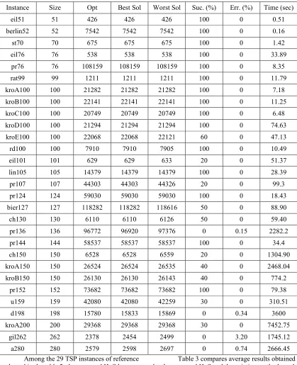
[image:6.595.87.294.183.578.2]Table 2: Numerical Results Obtained By Hus Applied To Some Tsp Instances Of Tsplib
Instance Size Opt Best Sol Worst Sol Suc. (%) Err. (%) Time (sec)
eil51 51 426 426 426 100 0 0.51
berlin52 52 7542 7542 7542 100 0 0.16
st70 70 675 675 675 100 0 1.42
eil76 76 538 538 538 100 0 33.89
pr76 76 108159 108159 108159 100 0 8.35
rat99 99 1211 1211 1211 100 0 11.79
kroA100 100 21282 21282 21282 100 0 7.18
kroB100 100 22141 22141 22141 100 0 11.25
kroC100 100 20749 20749 20749 100 0 6.48
kroD100 100 21294 21294 21294 100 0 74.63
kroE100 100 22068 22068 22121 60 0 47.13
rd100 100 7910 7910 7905 100 0 10.49
eil101 101 629 629 633 20 0 51.37
lin105 105 14379 14379 14379 100 0 28.39
pr107 107 44303 44303 44326 20 0 99.3
pr124 124 59030 59030 59030 100 0 18.43
bier127 127 118282 118282 118616 50 0 88.90
ch130 130 6110 6110 6126 50 0 59.40
pr136 136 96772 96920 97376 0 0.15 2282.2
pr144 144 58537 58537 58537 100 0 34.4
ch150 150 6528 6528 6559 20 0 1304.90
kroA150 150 26524 26524 26535 40 0 2468.04
kroB150 150 26130 26130 26143 40 0 774.2
pr152 152 73682 73682 73682 100 0 79.38
u159 159 42080 42080 42259 30 0 310.51
d198 198 15780 15833 15869 0 0.34 3600
kroA200 200 29368 29368 29368 30 0 7452.75
gil262 262 2378 2454 2499 0 3.20 1745.12
a280 280 2579 2598 2697 0 0.74 2666.45
[image:7.595.89.508.155.670.2]Among the 29 TSP instances of reference evaluated in the table 2, the proposed HuS has solved in a good duration 25 TSP instances. The percentage of error of the four unresolved TSP instances in less of 3600 seconds is only between 0.15% and 3.20%.
Table 3: The Average Results Obtained By Many Methods
Instance Opt HuS HS [18] ACO [22] & [23] PSO [20] GA [19]
eil51 426 426 426.3 430 [23] 436.9 429
berlin52 7542 7542 7542 7594 [22] 7832 -
st70 675 675 675 750 [22] 697.5 -
eil76 538 538 540.2 552.6 [23] 560.4 -
kroA100 21282 21282 21282 21457 [23] - 22141
According to the table, we can see that average results obtained by HuS are the best, comparing to the other methods.
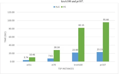
[image:8.595.90.508.294.554.2]Figure 8 compares average run times obtained by the methods HuS and HS for the four following Euclidean instances of TSP: eil51, st70, kroA100 and pr107.
Figure 8: The Average Run Time Obtained By Hus And Hs For Some Instances Of Tsp
According to the graph, we can clearly see that average run time obtained by HuS for the four instances of TSP are better than those of HS.
6. CONCLUSION
In the present paper, we have proposed an adaptation of the Hunting Search method to solve in an efficient way the combinatorial optimization problem; the TSP. Permutation operations were defined in order to achieve the adaptation as well as the simulation on TSPLib Library instances. This way helps to determine
the best parameters values of the HuS algorithm. The average of obtained optimum and the average of obtained run time of each instances are better compared to the recent methods such as Genetic Algorithm, Ant colony algorithm, Particle Swarm Optimization and Harmony Search, which encourage the use of Hunting Search method to solve similar problem.
3.74 7.61
22.00 23.13
10.46
28.18
82.15
95.66
0.00 20.00 40.00 60.00 80.00 100.00 120.00
eil51 st70 kroA100 pr107
T
IM
E
(
S
E
C
)
TSP INSTANCES
REFERENCES:
[1] APPLEGATE, David L. The traveling salesman problem: a computational study. Princeton University Press, 2006. [2] UNGUREANU, Valeriu. Traveling
Salesman Problem with Transportation. Computer Science, 2006, vol. 14, no 2, p. 41.
[3] FILIP, EXNAR et OTAKAR,
MACHAČ. The travelling salesman problem and its application in logistic practice. WSEAS Transactions on Business and Economics, 2011, vol. 8, no 4, p. 163-173.
[4] GOLDEN, Bruce L., RAGHAVAN, Subramanian, et WASIL, Edward A. The Vehicle Routing Problem: Latest Advances and New Challenges: latest advances and new challenges. Springer, 2008.
[5] ANDERSON, D. John. Optimal foraging and the traveling salesman. Theoretical Population Biology, 1983, vol. 24, no 2, p. 145-159.
[6] SHAKILA, Saad, WAN NURHADANI, Wan Jaafar, et SITI JASMIDA, Jamil. Solving standard traveling salesman problem and multiple traveling salesman problem by using branch-and-bound. 2013.
[7] KOLOMVOS, G., SAHARIDIS, G. K. D., et GOLIAS, M. M. Improvements in the Exact Solution Method for the Traveling Salesman Problem. In: Transportation Research Board 93rd Annual Meeting. 2014.
[8] PADBERG, Manfred et RINALDI, Giovanni. A branch-and-cut algorithm for the resolution of large-scale symmetric traveling salesman problems. SIAM review, 1991, vol. 33, no 1, p. 60-100.
[9] LIN, Shen et KERNIGHAN, Brian W. An effective heuristic algorithm for the traveling-salesman problem. Operations research, 1973, vol. 21, no 2, p. 498-516. [10] JOHNSON, David S. et MCGEOCH,
Lyle A. The traveling salesman problem: A case study in local optimization. Local search in combinatorial optimization, 1997, vol. 1, p. 215-310.
[11] VOUDOURIS, Christos et TSANG, Edward. Guided local search and its application to the traveling salesman
problem. European journal of operational research, 1999, vol. 113, no 2, p. 469-499.
[12] GENDREAU, Michel, LAPORTE, Gilbert, et SEMET, Frédéric. A tabu search heuristic for the undirected selective travelling salesman problem. European Journal of Operational Research, 1998, vol. 106, no 2, p. 539-545.
[13] SOAK, Sang-Moon et AHN, Byung-Ha. New genetic crossover operator for the TSP. In: Artificial Intelligence and Soft Computing-ICAISC 2004. Springer Berlin Heidelberg, 2004. p. 480-485. [14] GENG, Xiutang, CHEN, Zhihua, YANG,
Wei, et al. Solving the traveling salesman problem based on an adaptive simulated annealing algorithm with greedy search. Applied Soft Computing, 2011, vol. 11, no 4, p. 3680-3689.
[15] PURIS, Amilkar, BELLO, Rafael, MARTÍNEZ, Yailen, et al. Two-stage ant colony optimization for solving the traveling salesman problem. In : Nature Inspired Problem-Solving Methods in Knowledge Engineering. Springer Berlin Heidelberg, 2007. p. 307-316.
[16] TSAI, Cheng-Fa, TSAI, Chun-Wei, et TSENG, Ching-Chang. A new hybrid heuristic approach for solving large traveling salesman problem. Information Sciences, 2004, vol. 166, no 1, p. 67-81. [17] WONG, Li-Pei, LOW, Malcolm Yoke
Hean, et CHONG, Chin Soon. A bee colony optimization algorithm for traveling salesman problem. In: Proceedings of the 2008 Second Asia International Conference on Modelling & Simulation (AMS). IEEE Computer Society, 2008. p. 818-823.
[18] SHI, Xiaohu H., LIANG, Yanchun Chun, LEE, Heow Pueh, et al. Particle swarm optimization-based algorithms for TSP and generalized TSP.Information Processing Letters, 2007, vol. 103, no 5, p. 169-176.
[19] BOUZIDI, MORAD et RIFFI,
MOHAMMED ESSAID.
ADAPTATION OF THE HARMONY SEARCH ALGORITHM TO SOLVE
THE TRAVELLING SALESMAN
[20] OFTADEH, R., MAHJOOB, M. J., et
SHARIATPANAHI, M. A novel meta-heuristic optimization algorithm inspired by group hunting of animals: Hunting search. Computers & Mathematics with Applications, 2010, vol. 60, no 7, p. 2087-2098.