BIROn - Birkbeck Institutional Research Online
Paterson, Maura B. and Stinson, D.R. (2014) A unified approach to
combinatorial key predistribution schemes for sensor networks. Designs,
Codes and Cryptography 71 , pp. 433-457. ISSN 0925-1022.
Downloaded from:
Usage Guidelines:
Please refer to usage guidelines at or alternatively
BIROn -
B
irkbeck
I
nstitutional
R
esearch
On
line
Enabling open access to Birkbeck’s published research output
A unified approach to combinatorial key predistribution
schemes for sensor networks
Journal Article
http://eprints.bbk.ac.uk/5365
Version: Accepted (Refereed)
Citation:
© 2012
Springer
Publisher version
______________________________________________________________
All articles available through Birkbeck ePrints are protected by intellectual property law, including copyright law. Any use made of the contents should comply with the relevant law.
______________________________________________________________
Deposit Guide
Contact: [email protected]
Birkbeck ePrints
Birkbeck ePrints
Paterson, M.B. and Stinson, D.R. (2012)
A unified approach to combinatorial key predistribution schemes for
sensor networks –
A Unified Approach to Combinatorial Key Predistribution Schemes
for Sensor Networks
Maura B. Paterson
Department of Economics, Mathematics and Statistics Birkbeck, University of London
Malet Street, London WC1E 7HX, UK
Douglas R. Stinson∗
David R. Cheriton School of Computer Science University of Waterloo
Waterloo, Ontario, N2L 3G1, Canada
January 7, 2012
Abstract
There have been numerous recent proposals for key predistribution schemes for wireless sensor networks based on various types of combinatorial structures such as designs and codes. Many of these schemes have very similar properties and are analysed in a similar manner. We seek to provide a unified framework to study these kinds of schemes. To do so, we define a new, general class of designs, termed “partially balancedt-designs”, that is sufficiently general that it encompasses almost all of the designs that have been proposed for combinatorial key predistribution schemes. However, this new class of designs still has sufficient structure that we are able to derive general formulas for the metrics of the resulting key predistribution schemes. These metrics can be evaluated for a particular scheme simply by substituting appropriate parameters of the underlying combinatorial structure into our general formulas. We also compare various classes of schemes based on different designs, and point out that some existing proposed schemes are in fact identical, even though their descriptions may seem different. We believe that our general framework should facilitate the analysis of proposals for combinatorial key predistribution schemes and their comparison with existing schemes, and also allow researchers to easily evaluate which scheme or schemes present the best combination of performance metrics for a given application scenario.
1
Introduction
Awireless sensor network(WSN) is comprised of smallsensor nodesthat have very limited storage, power and computational capabilities. The nodes in a wireless sensor network should be able to communicate with each other in order to accumulate information and relay it to a base station in a secure manner. Because this communication often takes place in a hostile environment, encryption
∗
and/or authentication should be used. This requires the establishment of secure keys between the sensor nodes in the WSN.
One possible approach is to establish secret keys using public-key protocols such as key agree-ment schemes. However, for many examples of WSN, public-key cryptography is regarded as being unsuitable due to expensive computational costs [17]. A different approach, which is commonly considered for a WSN and which we follow in this paper, is to employ akey predistribution scheme
(orKPS), where secret keys are installed in each node before the sensor nodes are deployed. Two trivial examples of KPS can be considered. If every node is given the same secret “master key”, then memory costs are low. However, this situation is unsuitable because the compromise of a single node would render the network completely insecure. On the other hand, for every pair of nodes, there could be a secret pairwise key given only to these two nodes. This scheme would have excellent resiliency to node compromise, but memory costs would be prohibitively expensive for large networks because every node would have to store n−1 keys, where n is the number of nodes in the WSN.
The unsuitability of these two “extreme” KPS suggests that a suitable “intermediate” solution would be useful. In the seminal paper by Eschenauer and Gligor [17], a probabilistic approach to key predistribution for sensor networks is proposed: every node is assigned a random subset of keys chosen from a given pool of secret keys. The number of keys assigned to each node can be tailored to provide a good trade-off between various metrics of interest in the WSN (these metrics will be discussed in more detail in Section 1.4).
There have been dozens of papers that have investigated variations of this basic idea of assigning subsets of keys to nodes in a WSN. We briefly mention a few of these now.
• The basic Eschenauer-Gligor scheme [17] was generalized by Chan, Perrig and Song [12], who stipulated that two nodes will compute a pairwise key only if they share at least η
common keys, where the integer η is a pre-specified intersection threshold. Given that two nodes have at leastηcommon keys, they use all their common keys to compute their pairwise key, by means of an appropriate key derivation function (e.g., see Section 1.2). Roughly speaking, network connectivity decreases and resiliency increases asη is increased. Note that the Eschenauer-Gligor scheme is essentially the caseη= 1 of this more general approach.
• The use of deterministic methods in selecting subsets of keys for each node (as opposed to the random techniques used in [17] and elsewhere) has been investigated by a number of authors. Deterministic methods have some advantages as compared to randomised schemes; this is discussed in some detail in [24]. For example, security and connectivity properties of the schemes can be proven to hold in a deterministic scheme, whereas the desired properties may only hold with high probability in a randomised scheme. There are also performance advantages to some deterministic schemes (see Section 1.4). Constructions for deterministic KPS are usually based on combinatorial designs or error-correcting codes. This approach will be discussed in more detail in Section 1.1, and pertinent combinatorial designs will be treated in Section 1.5.
replaced by certain partial keying information for a corresponding “inner” scheme. If the inner scheme is a basic Blom scheme, this process would provide improved resiliency against node compromise, but at the same time it would increase the memory requirements by a factor of two.
In this paper, we will concentrate on KPS based on combinatorial designs (for a survey on this topic, see Martin [28]). We will utilise various intersection thresholds in the schemes we study, but we will not explicitly discuss multiple space schemes in this paper. However, we note that any subset-based scheme can easily be modified to yield a multiple space scheme. The use of multiple space schemes in a combinatorial setting was studied in [24], where it was concluded that it was a useful technique to improve the resilience of the resulting KPS.
1.1 Combinatorial Framework for Key Predistribution
In this section, we formally define the combinatorial framework we use in this paper. This framework is employed in several recent papers. We begin with the definition of a design.
Definition 1.1. A combinatorial design (or, more briefly, a design) is a pair (X,A), where A is
a finite set of subsets of X called blocks. The degree of a point x ∈ X is the number of blocks containing x. (X,A) is regular (of degree r) if all points have the same degree, r. The rank of
(X,A) is the size of the largest block. If all blocks have the same size, sayk, then (X,A) is said to be uniform (of rank k).
In this paper, we will mainly be making use of designs that are both regular and uniform.
Example 1.1. Let
X = {1,2,3,4,5,6,7,8,9}, and
A = {123,456,789,147,258,369,
159,267,348,168,249,357}.
Then (X,A) is a design in which there are nine points and twelve blocks. This design is regular of degree 4 and uniform of rank3.
Once the network size (denoted by b) and the number of keys per node (denoted by k) are specified, the centre chooses a regular, uniform design of rank k, say (X,A), having exactly b
blocks. The design (X,A) is used as thekey ring space. The key ring space will be used as a key predistribution scheme for a sensor network havingb nodes.
Let the sensor nodes be denoted U1, . . . , Ub. Let
X ={xi: 1≤i≤v}
and let
A={Aj : 1≤j≤b}.
The v points in X are associated with a set of v keys, as follows: For 1 ≤ i≤ v, a key, denoted by keyi, is chosen uniformly at random from some specified key-space, sayL (e.g., L ={0,1}128). Then, for eachj, 1≤j≤b, the sensor nodeUj receives the set ofk keys
We say that each point xi acts as the key identifier forkeyi, and we can view each block as a
set of key identifiers: the block Aj is used to identify the keys that are given to the node Uj. In
this model, the Eschenauer-Gligor scheme [17] is obtained when the key ring space is a set of n
randomk-subsets of thev-setX. A variation on this model is to use a key ring space withbblocks to set up a network with b0 nodes, whereb0 < b. In this case, we would randomly choose b0 of the
b blocks in the key ring space and use them to assign keys as described above. In the future, the network could be expanded if desired, by using additional blocks from the same key ring space to assign keys to new nodes which are added to the network.
1.2 Node Deployment Model
In the section, we discuss the standard node deployment model for WSN and how pairs of nodes construct pairwise keys. This requires use of the intersection threshold, denoted by η, that we mentioned earlier.
We assume that nodes are distributed randomly over a certain area, i.e., there is no precise control over where the nodes will end up. Two nodes N1 and N2 can construct a pairwise key to enable secure direct communication between them if and only if the following two conditions are satisfied:
(1) the two nodesN1 and N2 are within each other’s communication range, and
(2) the two nodesN1 and N2 have at leastη common keys.
Suppose thatUi and Uj have exactly`common keys, say{keya1, . . . ,keya`}, where a1 < a2<· · ·<
a` and `≥η. Then they can each compute the same pairwise secret key,
Ki,j =h(keya1 k. . .kkeya` kikj),
using an appropriate public key derivation function h, which has suitable input and output sizes. Such key derivation functions could be constructed from a secure cryptographic hash function.
Since the two properties enumerated above are independent, it is useful to define two graphs which together determine the connectivity of the network. Both these graphs have vertices defined by the b nodes in the network. The physical graph has an edge joining two nodes N1 and N2 whenever property (1) is satisfied, and the block graph has an edge joining two nodes whenever property(2)is satisfied. Thekey-sharing graph, which indicates when two nodes can communicate directly, is the intersection of the physical graph and the block graph.
Note that the block graph depends only on the key predistribution scheme that is used, while the physical graph depends only on the actual distribution of the nodes when they are deployed. Separating these two aspects of WSN allows us to concentrate on them independently. In this paper, we focus on properties of the WSN that can be determined by analysing the block graph, which in turn depend on combinatorial properties of the underlying scheme used for key predistribution. Thus, we will be ignoring the physical graph and therefore we will always use the termlinkto refer to a pair of nodes that comprise an edge in the block graph.
1.3 Attack Model
extracts the keys stored in them. Under the assumption that these nodes are then removed from the network, it is obvious that any links involving the compromised nodes are broken. However, a more pernicious consequence is that the compromise of certain nodes can also cause other links to be broken that do not directly involve the compromised nodes. More precisely, a link formed by two nodes corresponding to two blocks A1, A2, where |A1 ∩A2| ≥ η, will be broken if a node corresponding to a blockB 6∈ {A1, A2}is compromised, provided thatA1∩A2 ⊆B. More generally, if nodes corresponding to blocksB1, . . . , Bsare compromised, then a link corresponding to two other
blocks A1, A2 will be broken whenever
A1∩A2⊆
s [
i=1
Bi.
1.4 Metrics for Evaluating Key Predistribution Schemes
There are various metrics that quantify different performance and security aspects of a key pre-distribution scheme for a wireless sensor network. We summarise four of these metrics now in the case of combinatorial schemes that follow the framework in Section 1.1.
Network size
The maximum number of nodes in a wireless sensor network supported in a combinatorial key predistribution scheme is equal to the number of blocks, which we denote byb.
Storage requirements
The number of keys stored in each node is equal to k, which is the rank of the underlying design.
Network connectivity
Recall that two nodes have a common key when the corresponding blocks contain at leastη
common points, i.e., when they form an edge in the block graph. It is common to measure local connectivity of a network by computing the probability that a randomly chosen pair of nodes can compute a common key (see, for example, [12, 16, 24]). This probability will be denoted byPr1. It is obvious thatPr1 increases as η decreases.
Network resilience
Resilience against node capture is commonly measured by computing the probability that a random link is broken by the compromise of a set of s random nodes not in the link (see [12, 16, 24]), for suitable values ofs. We denote this probability by fail(s). For simplicity, we will primarily consider the value offail(1) in this paper.
Some authors measure resiliency differently, by also considering broken links directly involving the compromised nodes. We will discuss this issue in Section 4.1.1.
One of the fundamental problems in designing a KPS for a WSN is how best to trade off the metrics described above. Given a desired network size, it suffices to choose any design that has enough blocks to accommodate the number of desired nodes. Therefore, we will concentrate mainly on storage, connectivity, and resiliency.
• We can achieve optimal storage and connectivity by giving every node the same key; however, this scheme has no resiliency.
• Giving every pair of nodes a different key provides optimal connectivity and resiliency at the expense of requiring every node to storeb−1 keys, which may be a prohibitively large storage requirement.
• If we give every node a different key, we have low storage and high resiliency, but no connec-tivity at all (such a network is completely useless, of course).
It should be clear that the fundamental problem is to simultaneously obtain high connectivity and resilience with low storage requirements, where “high” and “low” depend on the specific application scenario under consideration.
There are a huge number of possible combinations of the triples (k,Pr1,fail(1)) for combinatorial schemes that have been proposed in the literature. As mentioned above, we wantPr1 to be large, but at the same time, we want fail(1) to be small. In [14], the ratio ρ=Pr1/fail(1) is considered for several classes of schemes. It is desirable for this ratio to be as large as possible. This provides a good single measure for the utility of a scheme, especially when the ratio can be parametrised by the value ofk.
We should also mention one other important aspect of WSN performance, namely shared-key discovery[17]. This refers to the method by which a node will learn the identifiers of the keys held by a neighbouring node, based on a succinct description of a node’s identity. The underlying algebraic structure of many combinatorial schemes facilitates efficient algorithms for shared-key discovery. In contrast, if a node is given a random subset of keys, shared-key discovery is inherently less efficient. These issues, and other related potential performance advantages of combinatorial schemes, are further discussed in [24].
1.5 Previous Related Work and Outline of the Paper
We have already mentioned that the study of key predistribution in WSN began with the seminal 2002 paper of Eschenauer and Gligor [17], which proposed a randomised key predistribution scheme. Deterministic schemes were suggested a couple of years later by different researchers [7, 20, 38]. Since then, numerous schemes have been advocated that are based on various types of combinatorial structures such as codes and designs. We give a sample of some of the types of schemes that have been proposed, in (roughly) chronological order. Unless otherwise indicated, the schemes use intersection threshold η= 1.
Projective planes
Using projective planes for KPS for WSN was suggested in 2004 by C¸ amtepe and Yener [7, 8] and independently by Lee and Stinson [20] (also see [11]).
Generalised quadrangles
These were suggested by in 2004 by C¸ amtepe and Yener [7, 8].
Configurations and common intersection designs
These were suggested in 2005 by Lee and Stinson [21, 22, 23, 24].
Transversal designs of strength 2
Transversal designs of strength 3
These were suggested in 2005 by Lee and Stinson [22, 24], using intersection thresholdη= 2.
Partially balanced incomplete block designs
These were suggested in 2007 by Ruj and Roy [33].
Inversive planes/spherical geometries
These were suggested in 2008 by Dong, Pei and Wang [15].
Orthogonal arrays
These were suggested in 2008 by Dong, Pei and Wang [14] (also see [39]).
Reed Solomon codes
These were suggested in 2008 by Ruj and Roy [14].
Mutually orthogonal latin squares
These were suggested in 2008 by Xu, Chen and Wang [39].
Rational normal curves in projective spaces
These were suggested in 2010 by Pei, Dong, and Rong [32].
All of the above papers deal with the basic model for key predistribution that we have presented earlier. However, there have also been situations where combinatorial structures have been proposed for more specialised types of WSN. One example is grid-based networks, where the nodes are deployed in a square or hexagonal grid. This additional deployment knowledge can be exploited through the use of distinct difference configurations and Costas arrays [1, 2]. Other papers that consider a combinatorial approach to grid-based networks include [35, 36]. Another specialised model for WSN concerns networks where nodes are deployed randomly in groups. In this setting, a scheme based on transversal designs has been proposed in [29].
It quickly becomes evident from reading the papers in the itemised list above that there is a great deal of similarity among many of them. Typically, formulas are developed for the metrics defined in Section 1.4 and then some data is tabulated. Sometimes comparisons are made with other schemes in the literature relating to one or more of the metrics. However, it can be difficult to get an overall picture as to how these schemes really compare with each other.
In some instances, identical schemes were published using different descriptions. For example, the Reed-Solomon code based scheme in [34] is identical to the earlier TD-based scheme proposed in [21], despite claims made in [34] that the two schemes are “different” (the schemes are easily seen to be identical, based on the equivalence of the underlying combinatorial objects; see Section 2.7). The scheme based on mutually orthogonal latin squares [39] is also basically another presentation of the same scheme.
There are other examples of two or more schemes that have very similar behaviour in terms of the metrics. Again this can be explained in terms of similarities of the underlying combinatorial structures used to construct the schemes, and we will discuss this further in later sections of the paper.
termed “partially balanced t-designs”, that is sufficiently general that it encompasses almost all of the designs that have been proposed for combinatorial key predistribution schemes. However, this new class of designs still has sufficient structure that we are able to derive general formulas for the metrics of the resulting key predistribution schemes. These metrics can be evaluated for a particular scheme simply by substituting appropriate parameters of the underlying combinatorial structure into our general formulas.
We also compare various classes of schemes based on different designs, and point out that some existing proposed schemes are in fact identical, even though their descriptions may seem different. We believe that our general framework should facilitate the analysis of proposals for combinatorial key predistribution schemes and their comparison with existing schemes, and also allow researchers to easily evaluate which scheme or schemes present the best combination of performance metrics for a given application scenario.
The rest of this paper is organized as follows. In Section 2, we discuss the necessary design-theoretic background. In Section 3, we derive some block-intersection properties of designs that will be used in later sections of the paper. In Section 4.1, we state and prove all the formulas for for computing the metrics of the resulting KPS. Applications of the formulas and comparisons of the resulting schemes is the subject of Section 4.2 and additional discussion is provided in Section 4.3. Finally, we summarise the contributions of the paper in Section 5.
2
Design-theoretic background
2.1 Partially Balanced t-designs
We will be studying KPS based on a general class of designs that includes many familiar types of designs as special cases. To the best of our knowledge, this is a new definition, though it has obvious similarities with other, previously defined classes of designs. The challenge here is to specify a class of designs that is sufficiently general that it includes almost all of the designs that have been proposed as combinatorial KPS, but sufficiently structured that general explicit formulas for the metrics of these schemes can be derived.
Let v, k, t be positive integers and let λi be a positive integer, for 0 ≤ i ≤ t−1. A t
-(v, k, λ0, . . . , λt−1)-partially balancedt-design(orPBt D) is a pair (X,A) that satisfies the following properties:
1. A is a set of k-subsets of X (elements of X are called points and members of A are called
blocks).
2. There are exactly λ0 blocks.
3. For 1≤i≤t−1, everyi-subset of points occurs in either 0 orλi blocks.
4. Fort≤i≤k, every i-subset of points occurs in either 0 or 1 blocks.
The number of blocks in the design,λ0, can also be denoted by b. We can assume that every point occurs in at least one block, so it then follows that every point occurs in exactlyλ1 blocks. Thus a partially balanced t-design is a design of degreer=λ1.
In the next subsections, we introduce various special types of designs that are partially balanced
2.2 Transversal Designs
Lett, n and kbe positive integers such thatt≤k≤n. A transversal design TD(t, k, n) is a triple (X,H,A), whereX is a finite set of cardinalitykn,His a partition ofXintokparts (calledgroups) of size nand Ais a set of k-subsets ofX (calledblocks), which satisfy the following properties:
1. |H∩A|= 1 for everyH ∈ Hand every A∈ A, and
2. every subset oftelements of X from tdifferent groups occurs in exactly one block in A.
Note that the parameter t is called thestrength of the transversal design. The following well-known result follows from simple counting.
Lemma 2.1. For 0≤ i≤t, any i points from different groups of a TD(t, k, n) occur together in
exactlyλi =nt−i blocks.
Corollary 2.2. Suppose (X,H,A) is a TD(t, k, n). Then (X,A) is a t-(v, k, λ0, . . . , λt−1)-PBt D
where v=knand λi=nt−i for 0≤i≤t−1.
We note that transversal designs are easy to construct for any desired value oft. The following well-known construction is originally due to Bush [6].
Theorem 2.3. [6] Suppose that q is a prime power, t≤min{q−1, k} and k≤q+ 1. Then there
exists a TD(t, k, q).
We will describe this construction later, using the language of orthogonal arrays; see Section 2.8.
2.3 t-designs
A t-(v, k, λ)-design is a pair (X,A) which satisfies the following properties:
1. Ais a set of k-subsets ofX (calledblocks)
2. Everyt-subset of points occurs in exactlyλblocks.
The following well-known result is proven in many textbooks, e.g., [37, Theorem 9.4].
Lemma 2.4. For 0≤i≤t, every i-subset of points in a t-design occurs in exactly
λi=
λ v−it−i
k−i t−i
(1)
blocks.
When λ= 1, we get a PBtD:
Corollary 2.5. Suppose(X,A)is at-(v, k,1)-design. Then(X,A)is at-(v, k, λ0, . . . , λt−1)-PBt D
where theλi’s are given by (1).
• A projective plane of order q is a 2-(q2+q+ 1, q+ 1,1)-design. Projective planes are known to exist for orders that are prime powers. These designs were proposed for use as KPS in [7, 8, 20].
• For any prime powerq and anyd≥2, there is a 3-(qd+ 1, q+ 1,1)-design which is termed a
spherical geometry. Spherical geometries were proposed for use as KPS in [15]. These designs are easy to construct; one well-known way is to take the blocks of the design to be the orbit ofFq∪ {∞}under the action of the group PSL(2, qd). When d= 2, the spherical geometries
are also known asinversive planes.
2.4 Generalised Quadrangles
An (s, t)-generalized quadrangle is a pair (X,A) that satisfies the following properties:
1. A is a set of (s+ 1)-subsets of X (elements of X are called points and members of A are calledlines).
2. Every point occurs on exactlyt+ 1 lines.
3. There are exactly λ0 blocks.
4. Every pair of points is on at most one line.
5. Given a line Land a point x 6∈L, there is a unique pointy∈L such that x and y occur on a line.
For information about generalised quadrangles, see Payne and Thas [30]. Well-known properties of generalised quadrangles immediately yield the following result:
Theorem 2.6. An (s, t)-generalized quadrangle is a 2-((st+ 1)(s+ 1), s+ 1, λ0, λ1)-PBt D where
λ0= (st+ 1)(t+ 1) andλ1 =t+ 1.
2.5 Configurations
A configuration is just a PBtD with t = 2. Therefore, generalised quadrangles, 2-designs and transversal designs with t= 2 are all examples of configurations. A special type of configuration, termed a common intersection design, has been defined for use in KPS; see [21, 22, 23, 24]. (The “common intersection” property concerns the existence of two-hop paths in the resulting WSN, which we do not consider in the present paper.)
2.6 Normal Rational Curves and Conics
A class of PBtD based on normal rational curves in projective spaces was described by Pei in [31]. We provide a summary of this approach now. Let q ≥ n be a prime power. A normal rational curve (orNRC) of PG(n, q) is a set of points that can be mapped by an element of PGL(n+ 1, q) into the set
{(δn, δn−1, . . . , δ,1) :δ∈GF(q)} ∪ {(1,0,0, . . . ,0)}.
An NRC contains q+ 1 points, no n+ 1 of which lie in any hyperplane of PG(n, q). (This can be seen by interpreting the coordinates of the points as the rows of a Vandermonde matrix.)
Lemma 2.7.
1. If q≥n+ 2, then there is a unique NRC through any set ofn+ 3points of PG(n, q) non+ 1
of which lie in a hyperplane, so λn+3= 1.
2. There are
λ0=q2n−2
n−2
Y
i=0
(qn+1−qi)
NRC in PG(n, q).
3. There are
λ1 =qn−1
n−1
Y
i=1
(qn+1−qi)
NRC through each point ofPG(n, q).
4. For r = 2,3, . . . , n, the number of NRCS through any set of r linearly independent points of
PG(n, q) is given by
λr = n Y
i=r
(qn+1−qi)(q−1)r−1
r−2
Y
i=2
(q−i).
5. The number of NRCS through any set of n+ 1 points of PG(n, q), no n+ 1 of which lie in a hyperplane, is
λn+1 = (q−1)n−1
n−1
Y
i=1
(q−i).
6. The number of NRCS through any set of n+ 2 points of PG(n, q), no n+ 1 of which lie in a hyperplane, is
λn+2=
n Y
i=2
(q−i).
Proof. For i = 0,1,2, . . . , n, a set of i linearly independent points span a space of dimension
i−1, so the number of ways of choosing an additional point that is not contained in this space is (qn+1−qi)/(q−1).
Given n+ 1 linearly independent points, without loss of generality their coordinates can be taken to be (1,0, . . . ,0),(0,1,0, . . . ,0), . . . , (0,0, . . . ,0,1). Then any n of these points span a hyperplane having the equation xi = 0 for some i ∈ {0,1,2, . . . , n}. The number of ways of
choosing an additional point such that non+ 1 of the resulting set of points lie in a hyperplane is thus equal to the number of ways of choosing a point that has no coordinate equal to zero, namely (q−1)n+1/(q−1) = (q−1)n.
Given n+ 2 points, no n+ 1 of which lie in a hyperplane, without loss of generality their coordinates can be chosen to be (1,0, . . . ,0), (0,1,0, . . . ,0), . . . ,(0,0, . . . ,0,1),(1,1,1, . . . ,1). A hyperplane through n of the first n+ 1 of these points has the equation xi = 0 for some i ∈
n+ 3 points, non+ 1 of which lie in a hyperplane, it is necessary (and sufficient) to choose a point with no zero coordinates, and in which no two of the coordinates are equal. There are
(q−1)(q−2)· · ·(q−n+ 1)/(q−1) =
n+1
Y
i=2 (q−i)
ways of doing this.
In order to count how many NRC pass through a given set of ipoints, it suffices to count the number of ways of adding points to the set until a set of n+ 3 points, no n+ 1 of which lie in a hyperplane, is obtained, then divide by nq+1+3−i−i, which is the number of ways of choosingn+ 3−i
further points from a given NRC.
Theorem 2.8. Let X be the set of points of PG(n, q), and let A be the set of NRC. Then (X,A)
is a t-(v, k, λ0, . . . , λt−1)-PBt D with t = n+ 3, v = q2+q+ 1, k = q+ 1 and where the λis are
established in Lemma 2.7.
When n= 2, an NRC is an irreducible conic in PG(2, q). In this case we have t= 5, and we obtain the following.
Corollary 2.9. Suppose thatq is a prime power. Then there is a 5-(q2+q+ 1, q+ 1, λ
0, . . . , λ4)
-PBt D where the λis are as follows:
λ0 =q5−q2,
λ1 =q4−q2,
λ2 =q3−q2,
λ3 =q2−2q+ 1,
λ4 =q−2.
2.7 Equivalence of Transversal Designs, Orthogonal Arrays and MDS Codes
Combinatorial schemes for KPS in WSN have been proposed that are based on transversal designs, orthogonal arrays, and maximum distance separable codes (MDS codes). However, these structures are all equivalent to each other in a very strong sense. Basically, they’re all the same thing! Here we briefly review these concepts and discuss their equivalence.
We have already given the definition of a TD(t, k, n). We define a (t, k, n)-orthogonal array (or (t, k, n)-OA) to be ak×nt array ofnsymbols, such that the restriction of the array to anyt rows
contains every possible column vector of thensymbols exactly once.
An (`, M, d, n)-code is a set of M `-tuples (called codewords) defined over an alphabet of n
symbols, such that the hamming distance between any two distinct codewords is at least d. The well-knownSingleton boundasserts thatd≤n−lognM+ 1; if equality occurs, the code is termed a maximum distance separable code (or MDS-code). The best-known examples of MDS codes are theReed-Solomon codes.
The following theorem states the equivalence of the above-defined objects. Its proof is straight-forward, but it seems to be difficult if not impossible to find a proof of all these equivalences in one place in the literature. Therefore, for completeness, we include a proof here.
1. a (k, M, d, n)-MDS-code;
2. a (t, k, n)-OA; and
3. a TD(t, k, n).
Proof. We first show that the hypothesised OA and code are equivalent. Given a (t, k, n)-OA, construct a code whose codewords are the nt columns of the OA. We will prove that this code is a (k, nt, d=n−t+ 1, n)-MDS-code. Suppose there exist two codewords whose hamming distance is at most n−t. Then these two codewords have identical entries at least t coordinates. This contradicts the assumption that the nt codewords form an orthogonal array.
Conversely, suppose we have a (k, nt, d=n−t+ 1, n)-MDS-code. Construct ak×nt array, say
D, whose columns are the codewords. Consider the restriction of Dto any subset oft=n−d+ 1 rows. Thentt-tuples obtained from the columns of the array in this restriction must all be different (otherwise, the distance of the code is less than d). Since there arent different t-tuples, it follows that every possible t-tuple occurs in exactly one column of the array in this restriction. Because this property holds for all possible subsets of t rows of the array D, it follows that we have a (t, k, n)-OA.
Now we show that the hypothesised TD and OA are equivalent. We first show how to construct a TD(t, k, n) from a (t, k, n)-OA. LetDbe a (t, k, n)-OA on symbol set{1, . . . , n}. Label the rows of Das 1, . . . , k, and label the columns of Das 1, . . . , nt. Define
X={1, . . . , n} × {1, . . . , k}.
For 1≤i≤k, define
Gi ={1, . . . , n} × {i},
and then define
G ={Gi: 1≤i≤k}.
For 1≤r ≤nt, define
Br={(D(i, r), i) : 1≤i≤k},
and define
B={Br: 1≤r ≤nt}.
Then it is essentially trivial to prove that (X,G,B) is a TD(t, k, n).
The construction can be reversed: given a TD(t, k, n), we can use it to construct a (t, k, n )-OA. Suppose (X,G,B) is a TD(t, k, n). By relabelling the points if necessary, we can assume that
X ={1, . . . , n} × {1, . . . , k} and G ={Gi : 1≤i≤k}, where Gi ={1, . . . , n} × {i} for 1≤i≤k.
For each block B ∈ B and for 1≤i≤k, let (i, bi)∈B∩Gi (recall that each block intersects each
group in a unique point). Then, for eachB ∈ B, form thek-tuple (b1, . . . , bk). Construct an array
A whose columns consist of all thesek-tuples; it is easy to see thatA is a (t, k, n)-OA.
same as the proof for t= 2, so in some sense it would probably not even be considered a separate result in the case t >2.
As a historical note, the earliest explicit statement of equivalence for t >2 that we could find was in Keith Martin’s 1991 PhD thesis [27, p. 32]. The earliest mention of this (that we are aware of) in a published paper is in a 1995 paper by Blanchard [3]. In fact, the earliest reference of any sort to TD with t >2 that we could find was in 1979 by Hanani [18].
In the case t= 2, there are additional equivalent structures. We do not define these structures here (for their definitions, see [13]), but we record the equivalences for completeness. Proofs of the following equivalences can be found in many textbooks, e.g., [25, Theorem 22.2] and [37, Theorem 6.44].
Theorem 2.11. The following are equivalent:
1. a net of order n and degree k;
2. k−2 mutually orthogonal latin squares of order n;
3. a (2, k, n)-OA; and
4. a TD(2, k, n).
In addition, we should mention that a projective plane of order n is equivalent to any of the structures listed in Theorem 2.11 when k=n+ 1.
In view of the equivalences of combinatorial structures discussed in this section, one should be careful when proposing a KPS based on one of these combinatorial structures. Not surprisingly, if two structures are equivalent, it usually turns out that the KPS constructed from them are also “equivalent” in a natural way, and the metrics of the resulting schemes will in fact be identical. This has in fact happened in several published papers, as we already mentioned in Section 1.5.
2.8 Bush’s Construction for Orthogonal Arrays
For historical interest, we briefly describe Bush’s 1952 construction for orthogonal arrays. The orthogonal arrays constructed in [6] are in fact (t, q+ 1, q)-OA, whereq is a prime power andt < q. We note that Bush’s construction predates by several years the corresponding construction for the MDS codes that are generally known as Reed-Solomon codes.
Let the elements of Fq be enumerated as αi, 0 ≤ i ≤ q −1. For every polynomial f(x) =
f0+f1x+· · ·+ft−1xt−1 ∈Fq[x] having degree at most t−1, we construct the (q+ 1)-tuple
(f(α0), . . . , f(αq−1), ft−1).
The resulting set ofqt (q+ 1)-tuples are taken to be columns of an array that can be shown to be
a (t, q+ 1, q)-OA.
3
Block Intersection Properties of PB
t
D
It turns out that the metrics of interest for a KPS constructed from a combinatorial design de-pend on block intersection properties of the design. A PBtD has very regular block intersection properties, for which we derive formulas in this section.
Suppose we have a t-(v, k, λ0, . . . , λt−1)-PBtD, (X,A). Let B ∈ A and suppose C ⊆ B with
|C|=i, where 0≤i≤t−1. Define
µ0(i) =|{A∈ A:A∩B=C}|.
We will develop formulas for µ0(i) (in doing so, it will clear that these formulas are independent of the particular choice ofB and C used to defineµ0(i)).
Given t−1 points on a block B, there are preciselyλt−1−1 further blocks that contain those
t−1 points. Since each of those blocks contain no further points ofB, we haveµ0(t−1) =λt−1−1. Given i points onB, where 0≤i < t−1, there areλi−1 further blocks that contain thosei
points. However, some of these blocks contain additional points ofB. In particular, givenjfurther points of B, where 1≤j≤t−1−i, by definitionµ0(i+j) of those blocks intersectB in precisely those i+j points. There are k−ij ways of selecting j additional points and hence µ0(i) satisfies the following recursion:
µ0(t−1) =λt−1−1,
µ0(i) =λi−1− t−1−i
X
j=1
k−i j
µ0(i+j) (t−2≥i≥0). (2)
Now we present a non-recursive formula to compute the µ0(i)’s.
Theorem 3.1. For any t-(v, k, λ0, . . . , λt−1)-PBt D, the following formula holds for 0≤i≤t−1:
µ0(t−i) =
i−1
X
j=0 (−i)j
k−t+i j
(λt−i+j−1). (3)
Proof. Assume (3) holds for µ0(t−1), µ0(t−2), . . . , µ0(t−i+ 1). Then, rewriting (2), we have:
µ0(t−i) =λt−i−1− i−1
X
j=1
k−t+i j
µ0(t−i+j),
=λt−i−1− i−1
X
j=1
k−t+i i−j
µ0(t−j),
=λt−i−1− i−1
X
j=1
k−t+i i−j
j−1 X
s=0 (−1)s
k−t+j s
(λt−j+s−1),
=λt−i−1− i−1 X j=1 j−1 X s=0 (−1)s
k−t+i i−j+s
i−j+s s
(replace swithj−sand collect like values ofλt−s)
=λt−i−1− i−1
X
s=1
i−1
X
j=s
(−1)j−s
k−t+i i−s
i−s j−s
(λt−s−1),
=λt−i−1− i−1
X
s=1
i−1−s X
j=0 (−1)j
k−t+i i−s
i−s j
(λt−s−1),
(use the binomial theorem)
=λt−i−1− i−1
X
s=1
(−1)(−1)i−s
k−t+i i−s
(λt−s−1),
(set j=i−s)
=λt−i−1 + i−1
X
j=1 (−1)j
k−t+i j
(λt−i+j−1),
=
i−1
X
j=0 (−1)j
k−t+i j
(λt−i+j −1).
Some block intersection properties of transversal designs were previously presented in [14]. The formulas in [14] are just the special case of the recursive formulas (2) we stated above, when
λi=nt−i.
In the case of transversal designs, it may be of interest to point out that there is an alternative approach to derive these formulas that makes use of known results. We have observed previously that a TD(t, k, n) is equivalent to an MDS code of lengthk and minimum distancek−t+ 1 over an alphabet of size n. The number of blocks of the transversal design that intersect a given block in precisely t−i points is equal to the number of codewords that have distance k−t+ifrom a given codeword, which in turn equals the number Ak−t+i of codewords that have weight k−t+i.
For an MDS code, this quantity is known to be given by
Ak−t+i =
k k−t+i
i−1 X
j=0 (−1)j
k−t+i j
(ni−j−1),
(see [19, Theorem 7.4.1], for example). Since there are k−tk+i
ways of choosingt−ispecific points of a given block, this gives
µ0(t−i) =
i−1
X
j=0 (−i)j
k−t+i j
(ni−j −1). (4)
4
Constructing KPS From PB
t
D
In this section we restrict our attention to KPS with intersection threshold η constructed from a
t-(v, k, λ0, . . . , λt−1)-PBtD. Here are some definitions of important quantities that will determine properties of the resulting KPS. As always, the blocks of the design correspond to the nodes in the resulting sensor network.
• Recall from Section 1.2 that a linkis a set of two blocks {A1, A2} such that|A1∩A2| ≥η.
• For an integer isuch that η ≤i≤ t−1, an i-link is a set of two blocks {A1, A2} such that
|A1∩A2|=i.
• A block A is contained in a link {A1, A2} if A∈ {A1, A2}. For η ≤i ≤t−1, let αi denote
the number ofi-links that a fixed blockA is contained in.
• A block A breaksa link{A1, A2} ifA6∈ {A1, A2}and A1∩A2 ⊆A. For η≤i≤t−1, let βi
denote the number ofi-links that a fixed blockAbreaks.
• Define β =Pt−i=1ηβi and α=Pt−i=η1α. Thus α is the total number of links that a fixed block
A is contained in andβ is the total number of links that a fixed blockA breaks.
• Let Li denote the total number of i-links and let L = Pt−1
i=ηLi denote the total number of
links.
• For a given i-link, let γi denote the number of nodes that break the given link.
• The probability that a random pair of nodes is a link is denoted byPr1.
• fail(1) is defined to be the probability that a random link is broken by the compromise of a random node not in the link.
4.1 Formulas for the Metrics
Now we state and prove some simple lemmas giving formulas for the quantities defined above.
Lemma 4.1. For η≤i≤t−1, it holds that
αi=
k i
µ0(i).
Proof. LetB be a block. There are ki
ways to chooseipointsC⊆B, and for each such choice of
C there are exactly µ0(i) blocksA such thatA∩B =C.
Lemma 4.2. For q≤i≤t−1, it holds that
βi =µ0(i)
λi
2 −1
k i
Proof. SupposeA is a block. The number ofi-links containingA is ki
µ0(i). For eachC⊆Awith
|C| =i, there are λi blocks that contain C, say BC,1, . . . , BCλi, one of which is the block A. For
each of these blocks BC,j, there are µ0(i) blocks that will form ani-link withBC,j. It follows that
the total number of i-links {B, B0}, where B ∩B0 = C, is λ
iµ0(i)/2, since each i-link is counted
twice in the above analysis. LettingC vary over all thei-subsets ofA, the number ofi-links whose intersection is ani-subset ofA is kiλiµ0(i)/2. Therefore, the number ofi-links that are broken by
A is
k i
λiµ0(i)
2 −
k i
µ0(i) =µ0(i)
λi
2 −1
k i
.
Lemma 4.3. For η≤i≤t−1, it holds that Li=bαi/2. Furthermore,L=bα/2.
Proof. Define
C={(A,{A1, A2}) :{A1, A2} is a link andA∈ {A1, A2}}.
By first choosingAand then choosing ani-link containingA, we have that|C|=bαi. On the other
hand, if we first choose a link{A1, A2} and then chooseA∈ {A1, A2}, we obtain
|C|= 2Li.
This shows that 2Li =bαi. Summing overi, we get 2L=bα.
Lemma 4.4. For η≤i≤t−1, it holds that
γi =λi−2.
Proof. SupposeA and B are blocks such that A∩B =C, where|C|=i. There are λi blocks that
contain C, including A and B. If we exclude A and B, the λi−2 remaining blocks are precisely
the blocks that break the link {A, B}. Therefore,γi =λi−2.
Lemma 4.5. The probability that ani-link is broken by a random node not in the link isγi/(b−2).
Proof. Suppose A and B are blocks such that A∩B =C, where |C|=i. There are b−2 blocks other than A andB, of whichγi break the link {A, B}.
Corollary 4.6. It holds that
fail(1) = 1
L(b−2)
t−1
X
i=η
Liγi.
Proof. For eachi,η≤i≤t−1, there are Li i-links. It was shown in Lemma 4.5 that everyi-link
is broken by a random node not in the link with probability γi/(b−2). Averaging over allLlinks,
the result follows.
We now establish a simpler alternative formula that can be used to compute fail(1).
Theorem 4.7. It holds that
fail(1) = β
Proof. We want to prove that
1
L(b−2)
t−1
X
i=η
Liγi=
β L−α,
or, equivalently,
(L−α)
t−1
X
i=η
Liγi=βL(b−2).
Using the fact that 2L=bα (from Lemma 4.3), it follows that
L(b−2)
L−α =b.
Therefore the equality to be proved can be written as
t−1
X
i=η
Liγi =βb. (5)
Define
D={(A,{A1, A2}) :{A1, A2} is a link andA1∩A2⊆A}.
By first choosing A and then choosing a link broken by A, we have that |D| =βb. On the other hand, if we first choose a link{A1, A2} and then chooseA such thatA breaks the link, we obtain
|D|=
t−1
X
i=η
Liγi.
Therefore, (5) holds and the proof is complete.
Theorem 4.8. It holds that
Pr1=
L
b
2
=
α b−1.
Proof. There are 2b
pairs of nodes, of which L are links, so it is clear that Pr1 = (Lb 2)
. Using the
fact that 2L=bα (from Lemma 4.3), we see that
L
b
2
=
α b−1.
4.1.1 Alternative Measures of Resiliency
also [15]) does not yieldfail(1) as we have defined it in Section 1.4. This formula in fact computes the quantity
α+β
L =
the number of links that a fixed block is contained in or breaks
the total number of links . (6)
For example, when t= 3, the value of fail(1) (as we have defined it) is
fail(1) = 3n
2−2n−4
(n3−2)(n+ 2),
whereas the value computed in [14, p. 828] using the formula (6) is
3
n(n+ 2).
Both of these values are approximately 3/n2, but they are not the same.
Of course one can define resiliency in various ways, but it makes things confusing when different definitions are used in different papers, and even more confusing when different definitions are used in different places in the same paper, without pointing out these differences.
4.2 Evaluating the Metrics for Various Schemes
It is straightforward to use the formulas developed in the previous sections to compute Pr1 and
fail(1) for schemes based on PBtD. The necessary steps are as follows:
1. Starting with theλi values (η≤i≤t−1), compute theµi values using Theorem 3.1.
2. Compute theαi,βi and Li values using Lemmas 4.1, 4.2 and 4.3, respectively.
3. Use Theorem 4.7 to computefail(1) and use Theorem 4.8 to computePr1.
We have mentioned the fundamental problem of trading off connectivity against resiliency. We want Pr1 to be large, but at the same time, we want fail(1) to be small. In [14], the ratio
ρ = Pr1/fail(1) is considered for several TD-based schemes. It is desirable for this ratio to be as large as possible. In [14], the value ofk is fixed to be n+ 1 and only the intersection ratio η = 1 is considered. We perform more general analyses for varying values of k and η, including some asymptotic analyses similar to [14].
The TD-based schemes and metrics we are considering involve two independent parameters, namely k and n. It is therefore convenient to write k = cn, where 0 < c ≤ 1, and consider the behaviour ofPr1,fail(1) and ρ as n→ ∞. Actually, for the schemes under investigation, we need to take k = Ω(n) (otherwise, Pr1 → 0 as n → ∞). When k = cn, it turns out that limn→∞Pr1 is a positive constant that depends on c. We also explicitly consider the special cases k= n and
k=n+ 1 for some TD-based schemes.
4.2.1 TD(2, k, n) with intersection threshold η= 1
It was first proposed in [21] to build a scheme from a TD(2, k, n) with intersection thresholdη= 1. In this scheme, we haveb=n2,α1=k(n−1),β1 =k n−21
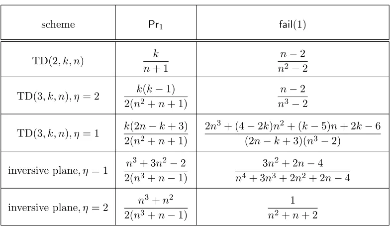
Table 1: Metrics for some PBtD-based schemes
scheme Pr1 fail(1)
TD(2, k, n) k
n+ 1
n−2
n2−2
TD(3, k, n), η = 2 k(k−1)
2(n2+n+ 1)
n−2
n3−2
TD(3, k, n), η = 1 k(2n−k+ 3) 2(n2+n+ 1)
2n3+ (4−2k)n2+ (k−5)n+ 2k−6 (2n−k+ 3)(n3−2)
inversive plane, η = 1 n
3+ 3n2−2
2(n3+n−1)
3n2+ 2n−4
n4+ 3n3+ 2n2+ 2n−4
inversive plane, η = 2 n 3+n2
2(n3+n−1)
1
n2+n+ 2
4.2.2 TD(3, k, n) with intersection threshold η= 2
This scheme was first proposed in [22]. Here, we haveb=n3,α2 = k2
(n−1), β2 = k2
n−1 2
, and
L2 = k2
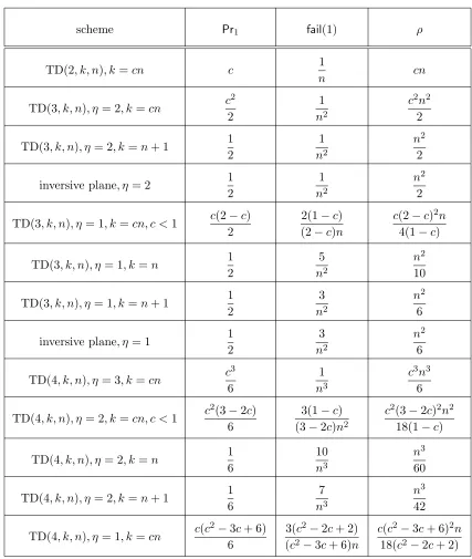
n3(n−1)/2. Exact values of Pr1 and fail(1) are given in Table 1. Asymptotic estimates of
Pr1,fail(1) andρ are listed in Table 2.
4.2.3 TD(3, k, n) with intersection threshold η= 1
This scheme was first proposed in [14]. Here, we have b = n3, α1 = k(n−1)(n−k+ 2), α2 =
k
2
(n−1), β1=k(n−1)(n−k+ 2)(n2−2)/2,β2 = k2
n−1 2
,L1 =n3k(n−1)(n−k+ 2)/2, and
L2 = k2
n3(n−1)/2. Exact values of Pr1 and fail(1) are given in Table 1. Asymptotic estimates of
Pr1,fail(1) andρ are listed in Table 2.
4.2.4 Comparing TD(3, n+ 1, n) to Inversive Planes
An inversive plane is a 3-(n2+ 1, n+ 1,1)-design. It is a 3-(n2 + 1, n+ 1, λ0, λ1, λ2)-PBtD where theλis are computed from (1) as follows:
λ0=n3+n,
λ1=n2+n,
λ2=n+ 1.
Table 2: Asymptotic values of metrics for some PBtD-based schemes
scheme Pr1 fail(1) ρ
TD(2, k, n), k=cn c 1
n cn
TD(3, k, n), η = 2, k=cn c
2
2
1
n2
c2n2
2
TD(3, k, n), η = 2, k=n+ 1 1
2
1
n2
n2
2
inversive plane, η= 2 1 2
1
n2
n2
2
TD(3, k, n), η= 1, k=cn, c <1 c(2−c) 2
2(1−c) (2−c)n
c(2−c)2n
4(1−c)
TD(3, k, n), η= 1, k=n 1
2
5
n2
n2
10
TD(3, k, n), η = 1, k=n+ 1 1
2
3
n2
n2
6
inversive plane, η= 1 1 2
3
n2
n2
6
TD(4, k, n), η = 3, k=cn c
3
6
1
n3
c3n3
6
TD(4, k, n), η= 2, k=cn, c <1 c
2(3−2c)
6
3(1−c) (3−2c)n2
c2(3−2c)2n2
18(1−c)
TD(4, k, n), η= 2, k=n 1
6
10
n3
n3
60
TD(4, k, n), η = 2, k=n+ 1 1
6
7
n3
n3
42
TD(4, k, n), η = 1, k=cn c(c
2−3c+ 6)
6
3(c2−2c+ 2) (c2−3c+ 6)n
c(c2−3c+ 6)2n
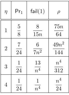
Exact values of Pr1 and fail(1) for inversive plane schemes, for different values of η, are given in Table 1. The asymptotic estimates of Pr1, fail(1) and ρ are presented in Table 3. We observe that these TD-based schemes have exactly the same asymptotic behaviour as the inversive plane schemes.
Table 3: Asymptotic values of metrics for TD(5, n+ 1, n) and NRC-PBtD (t= 5)
η Pr1 fail(1) ρ
1 5
8
8 15n
75n
64
2 7
24 6 7n2
49n2
144
3 1
24
13
n4
n4
312
4 1
24 1
n4
n4
24
4.2.5 TD(4, k, n)
For TD(4, k, n) and η = 1,2,3, we just provide the asymptotic estimates for Pr1,fail(1) and ρ in Table 2. (It is straightforward to work out the exact formulas, but they are quite complicated and the asymptotic estimates provide an easier way to summarise the behaviour of the schemes.)
4.2.6 Comparing TD(5, n+ 1, n) to NRC with t= 5
It is interesting to compare a scheme based on a TD(5, k, n) to a scheme constructed from an NRC-PBtD with t= 5 (Corollary 2.9). In the TD, we setk=n+ 1 so the block size is the same as in the NRC. We summarise the asymptotic estimates of Pr1,fail(1) andρ for different values of
η in Table 3. The interesting thing to note is that these TD-based schemes have exactly the same asymptotic behaviour as the NRC-based KPS.
4.3 Discussion
We believe that transversal designs (or any of the structures equivalent to them) offer the most flexibility of the PBtD-based schemes, due to several facts:
1. They are easy to construct for a wide variety of useful parameters, by using Bush’s construc-tion for orthogonal arrays, as described in Secconstruc-tion 2.8 (in this construcconstruc-tion, n can be any prime power).
3. In addition, the values oftandη can be chosen independently to best satisfy the constraints of a given application scenario.
It is worthwhile to investigate how changing the values of t,k,n, andη in a TD-based scheme affect the metrics of interest. Here are a few observations:
• In general, connectivity (i.e., the parameterPr1) is increased by increasing krelative tonor by decreasingη.
• Resilience increases as tis increased (i.e.,fail(1) decreases ast is increased). The ratioρ also increases ast increases.
• Complexity of the system increases as t is increased, since higher degree polynomials are required in order to construct the orthogonal arrays.
It is also of interest to comment on an interesting observation made in [14] concerning asymptotic values of ρ for orthogonal array schemes. It was observed for the parameters considered in [14] (namely, k =n+ 1 and η = 1) that ρ is O(n) except when t= 3, in which case ρ is O(n2). The computations we have shown in Table 2 explain this phenomenon. Basically, what happens is that, when we setk=cn, the value of ρcontains a factor of (1−c) in the denominator when η =t−2. If we set k=nor k=n+ 1 in these situations, then the value ofρ increases by a factor of O(n). Since [14] only considered η = 1, the consequence was that t = 3 ended up being an exceptional case in the data they computed.
5
Summary
We have presented a general and unified treatment of key predistribution schemes for wireless sensor networks based on combinatorial structures. We derived general formulas for the metrics of the resulting schemes and analysed several classes of schemes in detail. We believe that our general framework should facilitate the analysis of proposals for combinatorial key predistribution schemes and their comparison with existing schemes, and also allow researchers to easily evaluate which scheme or schemes present the best combination of performance metrics for a given application scenario. We also pointed out that many schemes presented in the literature as “different” schemes are in fact very similar and/or identical in some situations.
Acknowledgements
We would like to thank Simon Blackburn and Keith Martin for helpful discussions and comments.
References
[2] S.R. Blackburn, T. Etzion, K.M. Martin and M.B. Paterson. Distinct-difference configura-tions: multihop paths and key predistribution in sensor networks. IEEE Transactions on Information Theory 56(2010), 3961–3972.
[3] J.L. Blanchard. A construction for orthogonal arrays with strength t ≥ 3. Discrete Mathe-matics 137 (1995), 35–44.
[4] R. Blom. An optimal class of symmetric key generation systems. Lecture Notes in Computer Science 209 (1985), 335–338 (EUROCRYPT 1984).
[5] C. Blundo, A. De Santis, A. Herzberg, S. Kutten, U. Vaccaro and M. Yung. Perfectly secure key distribution for dynamic conferences.Information and Computation146 (1998), 1–23.
[6] K.A. Bush. Orthogonal arrays of index unity. Annals of Mathematical Statistics 23 (1952), 426–434.
[7] S. C¸ amtepe and B. Yener. Combinatorial design of key distribution mechanisms for wireless sensor networks.Lecture Notes in Computer Science3193(2004), 293–308 (ESORICS 2004).
[8] S. C¸ amtepe and B. Yener. Combinatorial design of key distribution mechanisms for wireless sensor networks.IEEE/ACM Trans. Networking 15 (2007), 346–358.
[9] D. Chakrabarti, S. Maitra and B. Roy. A key pre-distribution scheme for wireless sensor networks: merging blocks in combinatorial design.Lecture Notes in Computer Science 3650
(2005), 89–103 (ISC 2005).
[10] D. Chakrabarti, S. Maitra and B. Roy. A hybrid design of key pre-distribution scheme for wireless sensor networks. Lecture Notes in Computer Science 3803 (2005), 228–238 (ICISS 2005).
[11] D. Chakrabarti and J. Seberry. Combinatorial structures for design of wireless sensor net-works.Lecture Notes in Computer Science 3989(2006), 365–374 (ACNS 2006).
[12] H. Chan, A. Perrig, and D. Song. Random key predistribution schemes for sensor networks. In Proceedings of the 2003 Symposium on Security and Privacy. IEEE Computer Society, 197–213.
[13] C.J. Colbourn and J.H. Dinitz, eds. Handbook of Combinatorial Designs, Second Edition, Chapman & Hall/CRC, 2007.
[14] J.-W. Dong, D.-Y. Pei and X.-L. Wang. A class of key predistribution schemes based on orthogonal arrays. Journal of Computer Science and Technology23(2008), 825–831.
[15] J.-W. Dong, D.-Y. Pei and X.-L. Wang. A key predistribution scheme based on 3-designs.
Lecture Notes in Computer Science 4990(2008), 81–92 (Inscrypt 2007).
[17] L. Eschenauer and V. Gligor. A key-management scheme for distributed sensor networks. In
Proceedings of the 9th ACM Conference on Computer and Communications Security. ACM Press, 2002, pp. 41–47.
[18] H. Hanani. A class of three-designs.Journal of Combinatorial Theory A 26(1979), 1–19.
[19] W.C. Huffman and V. Pless.Fundamentals of Error-Correcting Codes, Cambridge University Press, 2003.
[20] J. Lee and D.R. Stinson. Deterministic key predistribution schemes for distributed sensor networks.Lecture Notes in Computer Science 3357(2005), 294–307 (SAC 2004).
[21] J. Lee and D.R. Stinson. A combinatorial approach to key predistribution for distributed sensor networks.IEEE Wireless Communications and Networking Conference (WCNC 2005), vol. 2, pp. 1200–1205.
[22] J. Lee and D.R. Stinson. On the construction of practical key predistribution schemes for distributed sensor networks using combinatorial designs. Technical Report CACR 2005-40, Centre for Applied Cryptographic Research, University of Waterloo, 2005.
http://www.cacr.math.uwaterloo.ca/techreports/2005/cacr2005-40.pdf.
[23] J. Lee and D.R. Stinson. Common intersection designs.Journal of Combinatorial Designs 14
(2006), 251–269.
[24] J. Lee and D.R. Stinson. On the construction of practical key predistribution schemes for distributed sensor networks using combinatorial designs. ACM Transactions on Information and System Security 11(2)(2008), article No. 1, 35 pp.
[25] J.H. van Lint and R.M. Wilson. A Course in Combinatorics, Second Edition. Cambridge, 2001.
[26] D. Liu, P. Ning and R. Li. Establishing pairwise keys in distributed sensor networks. ACM Transactions on Information and System Security 8 (2005), 41–77.
[27] K.M. Martin. Discrete Structures in the Theory of Secret Sharing, PhD thesis, University of London, 1991.
[28] K.M. Martin. On the applicability of combinatorial designs to key predistribution for wireless sensor networks.Lecture Notes in Computer Science 5557(2009), 124–145 (IWCC 2009).
[29] K.M. Martin, M.B. Paterson and D.R. Stinson. Key predistribution for homogeneous wireless sensor networks with group deployment of nodes.ACM Transactions on Sensor Networks 7-2
(2010), article No. 11, 27 pp.
[30] S.E. Payne and J. A. Thas.Finite Generalized Quadrangles, Second Edition.European Math-ematical Society Publishing House, 2009.
[31] D.-Y. Pei. Authentication Codes and Combinatorial Designs.Chapman & Hall/CRC, 2006.
[33] S. Ruj and B. Roy. Key predistribution schemes using partially balanced designs in wireless sensor networks.Lecture Notes in Computer Science 4742(2007), 431–445 (ISPA 2007).
[34] S. Ruj and B. Roy. Key predistribution schemes using codes in wireless sensor networks.
Lecture Notes in Computer Science 5487(2008), 275–288 (Inscrypt 2008).
[35] S. Ruj and B. Roy. Revisiting key predistribution using transversal designs for a grid-based deployment scheme.International Journal of Distributed Sensor Networks5(2008), 660–674.
[36] S. Ruj and B. Roy. Key predistribution using combinatorial designs for a grid-group deploy-ment scheme in wireless sensor networks.ACM Transactions on Sensor Networks6(1)(2009), article No. 4.
[37] D.R. Stinson. Combinatorial Designs, Constructions and Analysis. Springer, 2004.
[38] R. Wei and J. Wu. Product construction of key distribution schemes for sensor networks.
Lecture Notes in Computer Science 3357(2004), 280–293 (SAC 2004 Proceedings).