ISSN: 1992-8645 www.jatit.org E-ISSN: 1817-3195
( )
[
] [ ]
()!
t n
e
n
t
n
t
N
P
=
=
λ
−λDETECTION OF BURR TYPE III RELIABLE SOFTWARE
USING SPRT: AN ORDER STATISTIC APPROACH
1
K.SOBHANA, 2Dr. R. SATYA PRASAD, 3Dr. R. KIRAN KUMAR 1
Research Scholar, Department of Computer Science, Krishna University, Machilipatnam, India
2
Associate Professor, Department of CSE, Acharya Nagarjuna University, Guntur India
3
Assistant Professor& HOD, Department of CSE, Krishna University, Machilipatnam India
E-mail: [email protected] , [email protected],[email protected]
ABSTRACT
The acceptance of a software system depends on its reliability. Assessing reliability takes more time using classical hypothesis as the volume of data increases day by day. The volumes of data can be transformed using order statistics. Order statistics deals with applications of ordered random variables and functions of these variables. Sequential Analysis of Statistical science is very quick in deciding the reliability or unreliability on developed software. The method adopted is, Sequential Probability Ratio Test (SPRT) for continuous monitoring of the software. The likelihood based SPRT proposed by Wald is very general and it can be used for many different probability distributions. In this paper, the mean value function of Burr type III distribution based on Non-Homogenous Poisson Process (NHPP) with Order statistics and Sequential Probability Ratio Test is applied to analyze the results. Maximum Likelihood Estimation (MLE) is used to derive the unknown parameters of mean value function.
Keywords: Order Statistics, Software Reliability, Sequential Probability Ratio Test, Burr Type III, Maximum Likelihood Estimation
1. INTRODUCTION
Wald's procedure is particularly relevant if the data is collected sequentially. Sequential Analysis is different from Classical Hypothesis Testing where the number of cases tested or collected is fixed at the beginning of the experiment. In Classical Hypothesis Testing the data collection is executed without analysis and consideration of the data. After all data is collected the analysis is done and conclusions are drawn. However, in Sequential Analysis every case is analyzed directly after being collected, the data collected up to that moment is then compared with certain threshold values, incorporating the new information obtained from the freshly collected case. This approach allows one to draw conclusions during the data collection, and a final conclusion can possibly be reached at a much earlier stage as is the case in Classical Hypothesis Testing. The advantages of Sequential Analysis are easy to see as data collection can be terminated after fewer cases and decisions taken earlier.
In the analysis of software failure data, we often deal with either Time Between Failures or failure count in a given time interval. If it is further
assumed that the average number of recorded failures in a given time interval is directly proportional to the length of the interval and the random number of failure occurrences in the interval is explained by a Poisson process then we know that the probability equation of the stochastic process representing the failure occurrences is given by a Homogeneous Poisson Process (HPP) with the expression.
1 0
P P
( )
1 1
0 1
0 0
exp( )
N t
P
t P
λ
λ
λ
λ
= − +
1 0
P P
1
0
P
A
P
≥
1
0
P
B
P
≤
Concept of Order Statistics is given inSection2. The theory proposed by Stieber is described in Section 3. Implementation of SPRT for the proposed Burr type III Software Reliability Growth Model (SRGM) is illustrated in Section 4. Maximum Likelihood estimation method is used to estimate the unknown parameters is presented in Section 5. Analysis of the application of the SPRT on four data sets and conclusions drawn are given in Section 6 respectively.
2. ORDER STATISTICS
Order statistics deals with properties and applications of ordered random variables and of functions of these variables. The use of order statistics is significant when failures are frequent or inter failure time is less. Let X denote a continuous random variable with probability density function f(x) and cumulative distribution function F(x), and let (X1 , X2 , …, Xn) denote a random sample of size n drawn on X. The original sample observations may be unordered with respect to magnitude. A transformation is required to produce a corresponding ordered sample. Let (X(1) , X(2) , …, X(n)) denote the ordered random sample such that X(1) < X(2) < … < X(n); then (X(1), X(2), …, X(n)) are collectively known as the order statistics derived from the parent X. The various distributional characteristics can be known from Balakrishnan and Cohen [1]. The inter-failure time data is grouped into non overlapping successive sub groups of size 4 and 5 and add the failure times with in each sub group. The probability distribution of such a time lapse would be that of the rth ordered statistics in a subgroup of size ‘r’, which would be equal to power of the distribution function of the original variable [m(t)]. The order statistics is preferable when the failure data set is large. We implemented the Burr Type III model for 4th order and 5th order statistics.
3. WALD’S SEQUENTIAL PROBABILITY RATIO TEST FOR POISSON PROCESS
The Sequential Probability Ratio Test (SPRT) was developed by Abraham Wald at Columbia University in 1943[3]. The SPRT procedure is used for quality control studies during the manufacturing of software products. The tests can be performed on fixed sample size sets with fewer observations. The SPRT methodology for Homogeneous Poisson Process is described below.
Let {N(t), t ≥ 0} be a Homogeneous Poisson Process with rate ‘λ’. In this case, N(t) = number of failures up to time ‘t’ and ‘λ’ is the
failure rate (failures per unit time). If the system is put on test and that if we want to estimate its failure rate ‘λ’. We cannot expect to estimate ‘λ’ precisely. But we want to reject the system with a high probability if the data suggest that the failure rate is larger than λ1and accept it with a high probability,
if it is smaller than λ0. Here we have to specify two
(small) numbers ‘α’ and ‘β’, where ‘α’ is the probability of falsely rejecting the system. That is rejecting the system even if λ ≤ λ0. This is the
“producer’s” risk. ‘β’ is the probability of falsely accepting the system. That is accepting the system even if λ ≤ λ1. This is the “consumer’s” risk.
Wald‘s classical SPRT is very sensitive to the choice of relative risk required in the specification of the alternative hypothesis. With the classical SPRT, tests are performed continuously at every time point as t > 0 additional data are collected. With specified choices of λ0 and λ1 such that 0 < λ0
< λ1, the probability of finding N(t) failures in the
time span (0, t) with λ1, λ0 as the failure rates are
respectively given by
[ ]
( )1
1 1
( )!
N t te
t
P
N t
λ
λ
−
=
(1)
[ ]
( )0 0 0
( )!
N t t
e
t
P
N t
λ
λ
−
=
(2)
The ratio at any time ‘t’ is considered as a measure of deciding the truth towards or , given a sequence of time instants say
1 2 3 . . . K
t < t < t < < t and the corresponding
realizations of N(t)
Simplification of gives
The decision rule of SPRT is to decide in favor of , in favor of or to continue by observing the number of failures at a later time than ‘t’ accordingly as is greater than or equal to a constant say A, less than or equal to a constant say B or in between the constants A and B. That is, we decide the given software product as unreliable, reliable or continue[3] the test process with one more observation in failure data, according to
(3)
(4)
0
λ λ1
1 0
P P
1 2
( ) , ( ) , ... ( K)
N t N t N t
1
ISSN: 1992-8645 www.jatit.org E-ISSN: 1817-3195
α
β
1
0
P B P ≤ (5)
The approximate values of the constants A and B are taken as
, B
Where ‘ ’ and ‘ ’ are the risk probabilities as defined earlier. A simplified version of the above is:
To reject the system as unreliable if N(t) falls for the first time above the line
(6)
To accept the system to be reliable if N(t) falls for the first time below the line
(7)
To continue the test with one more observation on [t , N(t)] as the random graph of [t , N(t)] is between the two linear boundaries given by equations (6) and (7) where
(8)
(9)
(10)
The parameters , and can be chosen in several ways. One way suggested by Stieber is
,
If λ0 and λ1 are chosen in this way, the
slope of NU (t) and NL (t) equals λ. The other two
ways of choosing λ0 and λ1 are from past projects
(for a comparison of the projects) and from part of the data to compare the reliability of different functional areas (components).
4. SEQUENTIAL TEST FOR SOFTWARE RELIABILITY GROWTH MODELS
We know that for any Poisson process, the expected value of N(t) = λ(t) called the average number of failures experienced in time 't'. Which is also called the mean value function of the Poisson process. On the other hand if we consider a Poisson process with a general function (not necessarily linear) m(t) as its mean value function the probability equation of a such a process is
Depending on the forms of m(t) we get various Poisson processes called NHPP, for the Burr Type III model. The mean value function is given as
( )
[
]
b c
t a t
m = 1+ − −
It can also be written as
[
]
1( ) ( )
1 1
.
( )
( )!
N t m t
e
m t
P
N t
−
=
[
]
0( ) ( )
0 0
.
( )
( )!
N t m t
e
m t
P
N t
−
=
Where m1(t), m0(t) represents the mean
value function of stated parameters indicating reliable software and unreliable software respectively. The mean value function m(t) comprises the parameters ‘a’, ‘b’ and ‘c’. The two specifications of NHPP for b are considered as b0,
b1 where (b0 < b1) and two specifications of c say
c0, c1where (c0 < c1). For our proposed model, m(t)
at b1 is said to be greater than b0 and m(t) at c1 is
said to be greater than c0. The same can be denoted
symbolically as m0(t) < m1(t). The implementation
of SPRT procedure is illustrated below.
System is said to be reliable and can be accepted if
i.e.,
1
0
P
B
A
P
<
<
( )
.
2U
N
t
=
a t
+
b
( )
.
1L
N
t
=
a t
−
b
1 0
1
0
log
a
λ λ
λ
λ
−
=
1
1
0
1
log
log
b
α
β
λ
λ
−
=
2
1
0
1
log
log
b
β
α
λ
λ
−
=
,
α β
λ
0λ
1( )
0
.log
1
q
q
λ
λ
=
−
( )
1
.log
1
q
q
q
λ
λ
=
−
1
0
where q
λ
λ
=
[
] [
( )]
( )( ) . , 0,1, 2,
! y
m t
m t
P N t Y e y
y
−
= = = − − − −
[
]
[
]
1
0
( ) ( )
1
( ) ( )
0
.
( )
.
( )
N t
m t
N t
m t
e
m
t
B
e
m
t
−
(
)
(
)
(
)
(
)
(
)
(
)
(
)
(
)
− − − − − − − − − − − − − − − − − − − − 0 1 0 1 0 1 0 1 1 1 log 1 1 1 log 1 1 log 1 1 1 log b 0 c b 1 c b 0 c b 1 c b 0 c b 1 c b 0 c b 1 c t + t + t + t + a + α β < N(t) < t + t + t + t + a + α β(
)
(
)
rb c i t a t
m( ) = 1+( )− −
i.e., (11)
System is said to be unreliable and rejected if
i.e., (12)
Continue the test procedure as long as
(13)
Substituting the appropriate expressions of the respective mean value function, we get the respective decision rules and are given in followings lines. Acceptance Region (14) Rejection Region: (15) Continuation Region: (16)
For the specified model, it may be observed that the decision rules are exclusively based on the strength of the sequential procedure (α, β) and the value of the mean value functions namely m0(t) m1(t). As described by Stieber, these decision rules become decision lines if the mean value function is linear in passing through origin, that is m(t) = λt. The equations (11) and (12) are considered as generalizations for the decision procedure of Stieber. SPRT procedure is applied on live software failure data sets and the results that were analyzed are illustrated in Section 6.
5. PARAMETER ESTIMATION
We present expressions for the parameter estimates of the Burr type III model. Parameter estimation is very significant in software reliability prediction. Once the analytical solution form is known for a given model, parameter estimation is achieved by applying a well-known estimation, Maximum Likelihood Estimation (MLE).The main idea behind Maximum Likelihood parameter assessment is to decide the parameters that maximize the probability (likelihood) of the specimen data. In the other words, MLE methods are versatile and applicable to most models and for
different types of data. Here parameters are estimated from the time domain data [5].
The mean value function of Order Burr Type III is given as
(17)
The constants a, b and c in the mean value function are called parameters of the proposed model. To assess the software reliability, it is necessary to compute the expressions for finding the values of a, b and c. For doing this, Maximum Likelihood estimation is used whose Log Likelihood Function(LLF) is given by
LLF= i r n r
n
i
t
m
t
Log
[
(
)
(
)
1
−
∑
=
λ
(18)Differentiating m(t) with respect to ‘t’ we get (t)
λ
(t)= (19)1 0
1 0
l o g ( ) ( )
1 ( )
l o g ( ) l o g ( )
m t m t
N t
m t m t
β α + − − ≤ − 1 0
P
A
P
≥
1 0 1 0 1lo g ( ) ( )
( )
lo g ( ) lo g ( )
m t m t
N t
m t m t
β α − + − ≥ −
1 0 1 0
1 0 1 0
1
log ( ) ( ) log ( ) ( ) 1
( )
log ( ) log ( ) log ( ) log ( )
m t m t m t m t
N t
m t m t m t m t
β β
α α
−
+ − + −
−
< <
− −
(
)
(
)
(
)
(
)
(
)
+ + + − + + − ≤ − − − − − − − − 0 0 1 1 0 0 1 1 1 1 log 1 1 1 log ) ( b c b c b c b c t t t t a t N α β(
)
(
)
(
)
(
)
− − ≥ − − − − − − − − 0 1 0 1 1 1 log 1 1 1 log b 0 c b 1 c b 0 c b 1 c t + t + t + t + a + α β N(t)λ
) 1 ( ) 1 (]
)
(
1
[
*
)
(
++
i −c br+ ci
t
t
ISSN: 1992-8645 www.jatit.org E-ISSN: 1817-3195 ) 0 log = ∂ ∂ a L
r
t
n
(
1
+
(
n)
−c)
br) ) ( 1 ( log . ) ) ( 1
( 1 2 1
2 2 − − + + + − n br n t t n b n ) 0 log = ∂ ∂ c L ) ( ' ) ( b = bn+1 n
n n b g b g
)
(
'
)
(
-c
=
c
n+1 nn n
c
g
c
g
The log likelihood equation to estimate the unknown parameters a, b, c after substituting (19) in (18) is given by
LogL=-[a[1+(tn)-c]-b]r + +
(20)
Differentiating LogL with respect to ‘a’
and equating to 0 (i.e., we get
ar = (21)
Differentiating LogL with respect to ‘b’ and equating to 0 (i.e., we get
g(b)= (22)
Again Differentiating g(b) with respect to ‘b’ and equating to 0 (i.e., we get
g'(b) = (23)
Differentiating LogL with respect to ‘c’ and equating to 0(i.e., we get
g(c) = (24)
Again Differentiating g(c) with respect to ‘c’ and equating to 0 (i.e., we get
g'(c) = (25)
The parameters ‘b’ and ‘c’ are estimated by iterative Newton-Raphson Method using
(26)
(27)
which are substituted in (21) to determine ‘a’.
6. SPRT ANALYSIS OF LIVE DATASETS
In this section, the SPRT methodology is applied on four different data sets for 4th ordered and 5th ordered statistics referred from (LYU 1996)] and the decisions are evaluated on the mean value function.
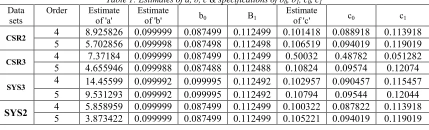
The specifications for parameters b0, b1
and c0, c1 are chosen on the parameter estimates b
and c as b0 = b – δ, b1 = b + δ and c0 = c – δ, c1 = c
+δ, and apply SPRT such that b0 < b < b1 and c0 < c
< c1. Assuming the δ value of 0.0125 the choices
are given in Table 1.
Using the specification b0, b1, and c0, c1
the mean value functions m0(t) and m1(t) are
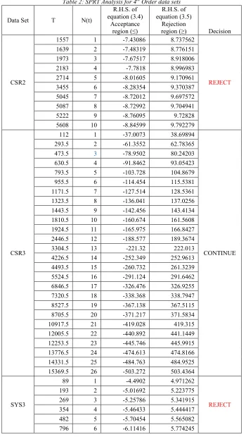
[image:5.612.92.521.610.740.2]computed for each ‘t’. Later the decisions are made based on the decision rules specified by the equations (14), (15), (16) for the data sets. At each ‘t’ of the data set, the strengths (α, β) are considered as (0.6, 0.6). SPRT procedure is applied on four different data sets and the necessary calculations are given in Table 2 and Table 3.
Table 1: Estimates of a, b, c & specifications of b0, b1, c0, c1
Data sets
Order Estimate of 'a'
Estimate
of 'b' b0 B1
Estimate
of 'c' c0 c1
CSR2 4 8.925826 0.099999 0.087499 0.112499 0.101418 0.088918 0.113918
5 5.702856 0.099998 0.087498 0.112498 0.106519 0.094019 0.119019
CSR3 4 7.37184 0.099999 0.087499 0.112499 0.50032 0.48782 0.051282
5 4.655946 0.099988 0.087488 0.112488 0.10824 0.09574 0.12074
SYS3 4 14.45599 0.099992 0.099995 0.112492 0.102957 0.090457 0.115457
5 9.531293 0.099992 0.099995 0.112492 0.10794 0.09544 0.12044
SYS2 4 5.858959 0.099999 0.087499 0.112499 0.100322 0.087822 0.113918
5 3.873422 0.099999 0.087499 0.112499 0.105221 0.094019 0.119019
∑
= + + + n i c b a r 1 ] log log log [log∑
− − − + + + − n i i ci c t
t br 1 )] log( ) 1 ( ) ) ( 1 log( ) 1 ( [ ) 0 log = ∂ ∂ b L ) ) ( 1 log( ) ) ( 1 ( ) ) ( 1 log( 1 1 2 1
1 − −
=
− + + +
+
+
∑
nTable 2: SPRT Analysis for 4th Order data sets
Data Set T N(t)
R.H.S. of equation (3.4)
Acceptance region (≤)
R.H.S. of equation (3.5)
Rejection
region (≥) Decision
CSR2
1557 1 -7.43086 8.737562
REJECT 1639 2 -7.48319 8.776151
1973 3 -7.67517 8.918006 2183 4 -7.7818 8.996983 2714 5 -8.01605 9.170961
3455 6 -8.28354 9.370387 5045 7 -8.72012 9.697572 5087 8 -8.72992 9.704941 5222 9 -8.76095 9.72828 5608 10 -8.84599 9.792279
CSR3
112 1 -37.0073 38.69894
CONTINUE 293.5 2 -61.3552 62.78365
473.5 3 -78.9502 80.24203 630.5 4 -91.8462 93.05423 793.5 5 -103.728 104.8679 955.5 6 -114.454 115.5381 1171.5 7 -127.514 128.5361
1323.5 8 -136.041 137.0256 1443.5 9 -142.456 143.4134 1810.5 10 -160.674 161.5608 1924.5 11 -165.975 166.8427 2446.5 12 -188.577 189.3674 3304.5 13 -221.32 222.013
4226.5 14 -252.349 252.9613 4493.5 15 -260.732 261.3239 5524.5 16 -291.124 291.6462 6846.5 17 -326.476 326.9255 7320.5 18 -338.368 338.7947
8527.5 19 -367.138 367.5115 8705.5 20 -371.217 371.5834 10917.5 21 -419.028 419.315 12005.5 22 -440.892 441.1449 12253.5 23 -445.746 445.9915 13776.5 24 -474.613 474.8166
14331.5 25 -484.763 484.9525 15369.5 26 -503.272 503.4364
SYS3
89 1 -4.4902 4.971262
REJECT 193 2 -5.01692 5.223775
269 3 -5.25786 5.341915 354 4 -5.46433 5.444417
ISSN: 1992-8645 www.jatit.org E-ISSN: 1817-3195
SYS2
1576 1 -6.21469 8.445398
REJECT 4149 2 -7.05728 9.121103
5827 3 -7.3793 9.38095 10071 4 -7.92966 9.826981
11836 5 -8.09994 9.965455 15280 6 -8.37693 10.19115 16860 7 -8.48622 10.28036 19572 8 -8.65469 10.41803 23827 9 -8.88216 10.60423
[image:7.612.91.516.67.724.2]28257 10 -9.08434 10.77001 31886 11 -9.23047 10.89001
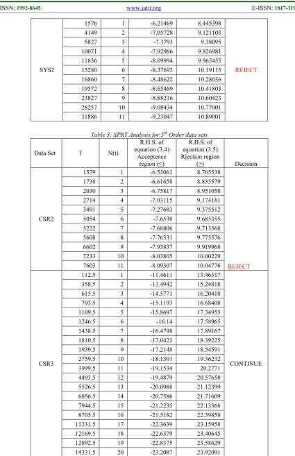
Table 3: SPRT Analysis for 5th Order data sets
Data Set T N(t)
R.H.S. of equation (3.4)
Acceptence region (≤)
R.H.S. of equation (3.5) Rjection region
(≥) Decision
CSR2
1579 1 -6.53061 8.765538
REJECT 1738 2 -6.61658 8.835579
2030 3 -6.75817 8.951058 2714 4 -7.03115 9.174181 3491 5 -7.27683 9.375512
5054 6 -7.6538 9.685355 5222 7 -7.68806 9.713568 5608 8 -7.76331 9.775576 6602 9 -7.93837 9.919968 7233 10 -8.03805 10.00229 7603 11 -8.09307 10.04776
CSR3
112.5 1 -11.4611 13.46317
CONTINUE 358.5 2 -13.4942 15.24818
615.5 3 -14.5771 16.20418 793.5 4 -15.1193 16.68408 1109.5 5 -15.8697 17.34955
1246.5 6 -16.14 17.58965 1438.5 7 -16.4798 17.89167 1810.5 8 -17.0423 18.39225 1939.5 9 -17.2148 18.54591 2759.5 10 -18.1301 19.36232 3999.5 11 -19.1534 20.2771
4493.5 12 -19.4879 20.57658 5526.5 13 -20.0988 21.12399 6856.5 14 -20.7586 21.71609 7944.5 15 -21.2235 22.13368 8705.5 16 -21.5182 22.39858 11231.5 17 -22.3639 23.15958
SYS3 93 1 -5.79193 1.76024 REJECT 243 2 -5.99538 1.818877
SYS2
2610 1 -12.9566 15.54412
CONTINUE 4436 2 -13.9495 16.4418
8163 3 -15.2031 17.57807 11836 4 -16.0317 18.33066 15685 5 -16.6951 18.93413 17995 6 -17.0305 19.23954 22226 7 -17.5618 19.72358
28257 8 -18.1897 20.29631 32346 9 -18.5549 20.62965 39856 10 -19.1364 21.16074 46147 11 -19.5574 21.54566 53223 12 -19.978 21.93028 58996 13 -20.2882 22.2142
67374 14 -20.6968 22.58828 80106 15 -21.2442 23.0898 91190 16 -21.6653 23.47592 98692 17 -21.9272 23.71607
7. CONCLUSION
The SPRT methodology for the proposed software reliability growth model Burr type III is applied for four software failure data sets. This model has given a decision of rejection for 3 data sets i.e., CSR2, SYS3 and SYS2 at 10th ,6thand 11th instances respectively ,a decision of continue for 1 data set i.e., CSR3 using 4th order .It has given a decision of rejection for 2 datasets i.e., CSR2 and SYS3 at 11th and 2nd instances respectively, a decision of continue for 2 data sets i.e., CSR3 and SYS2 using 5th order. Hence, it is observed that we are able to come to a conclusion in less time regarding the reliability or unreliability of a software product by applying SPRT.
REFERENCES:
[1] Balakrishnan, N. and Cohen, A.C., (1991). “Order statistics and inference: estimation methods”, Academic Press.
[2] Wald. A., (1945). “Sequential tests of statistical hypotheses”. Annals of Mathematical Statistics, 16:117– 186.
[3] Wald A. “Sequential Analysis”. New
Impression edition. New York: John Wiley and Son, Inc; 1947 Sep 30.
[4] STIEBER, H.A.(1997). “Statistical Quality Control: How To Detect Unreliable Software
Components”, Proceedings the 8th
International Symposium on Software
Reliability Engineering, 8-12
[5] K.Sobhana, Dr.R.Satya Prasad, Ch.Smitha Chowdary, “Software Reliability Growth Model on Burr Type III-An Order Statistics Approach”, International Journal of Software Engineering, IJSE Vol.8 No.1 January 2015. [6] G. Sridevi Gutta, Dr. R. Satya Prasad,
“Detection of Reliable Pareto Software Using SPRT”, IJCSI International Journal of Computer Science Issues, Vol. 11, Issue 1, No 1, January 2014.
[7] Dr. R. Satya Prasad, Mrs. Srisaila, Dr. G. Krishna Mohan, “Software Reliability Using
SPRT: Power Law Process Model”,
International Journal of Electronics and Computer Science Engineering, IJECSE, Volume 3, Number 4, ISSN- 2277-1956. [8] K. Sita Kumari, Dr. R. Satya Prasad, “Pareto
Type II Software Reliability Growth Model–An Order Statistics Approach”, International Journal of Computer Science Trends and Technology (IJCST) Volume 2Issue 4,Jul-Aug 2014.
ISSN: 1992-8645 www.jatit.org E-ISSN: 1817-3195
[10] Dr. R. Satya Prasad, K. Syed, T. Anuradha “Rayleigh based SPRT: Order Statistics”, IJCERT International Journal of Computer Engineering In Research Trends, Volume 2, Issue 8, August-2015, pp. 523-529.
[11] D. Haritha, Dr. R. Satya Prasad, “Detecting Reliable Software Using SPRT: An Order Statistics Approach”, IJCST Vol. 4, Issue 2, April - June 2013.
[12] Chansoo Kim, Seongho Song, Woosuk Kim, “Statistical Inference for Burr Type III Distribution on Dual Generalized Order Statistics and Real Data Analysis”, Applied Mathematical Sciences, Vol. 10, 2016, no. 14, 683 - 695
[13] K. V. Murali Mohan, R. Satya Prasad , G. Sridevi, “Detection of Burr Type XII Reliable Software using Sequential Process Ratio Test”, Indian Journal of Science and Technology, ISSN: 0974 -5645, Vol.8. Issue16,July 2015. [14] K.B.Misra. “Handbook of Performability
Engineering”. Springer. 2008.
[15] Ch.Smitha Chowdary, Dr R. Satya Prasad, K. Sobhana, “Burr Type III Software Reliability Growth Model,” IOSR-JCE Volume17, Issue 1, Jan-Feb 2015
[16] Pham H. System Software Reliability. Springer; 2006.
[17] Lyu MR.The Hand book of software Reliability engineering. McGrawHill and IEEE Computer Society Press; 1995. ISBN: 9-07-039400-8.
[18] Ashoka M. Data set. Bangalore: Sonata Software Limited; 2010.
[19] I.W. Burr and P.J. Cislak, “On a general system of distributions: I. Its curve-shape characteristics; II The sample median”, Journal of the American Statistical Association, 63 (1968), 627-635.
[20] N.L. Johnson, S. Kotz and N. Balakrishnan, “Continuous Univariate Distributions”, 2nd edition, John Wiley & Sons, New York, USA, 1995.
[21] Dr. R. Satya Prasad, V. Suryanarayana, Dr. G. Krishna Mohan , “GOMPERTZ BASED SPRT: MLE”, JATIT Journal of Theoretical and Applied Information Technology, Vol.86. No.2, 20 April 2016.