A Comparison between two Modified NSGA-II
Algorithms for Solving the Multi-objective Flexible Job
Shop Scheduling Problem
Aydin Teymourifar
1,2,∗,
Gurkan Ozturk
1,2,
Ozan Bahadir
1,21Faculty of Engineering, Anadolu University, 26555, Eskisehir, Turkey
2Computational Intelligence and Optimization Laboratory (CIOL), Anadolu University, 26555, Eskisehir, Turkey
Copyright c2018 by authors, all rights reserved. Authors agree that this article remains permanently open access under the terms of the Creative Commons Attribution License 4.0 International License
Abstract
Many evolutionary algorithms have been used to solve multi-objective scheduling problems. NSGA-II is one of them that is based on the Pareto optimality concept and generally obtains good results. However, it is possible to improve its performance with some modifications. In this paper, two modified NSGA-II algorithms have been suggested for solving the multi-objective flexible job shop scheduling problem. The neighborhood structures defined for the problem are integrated into the algorithms to create better generations during the iterations. Also, their initial populations are created with an effective heu-ristic. In the first modified NSGA-II, after the creation of the offspring population, a neighbor of each individual in the parent population is constructed, and then one of them is selected according to the domination state of the solutions. Then the popula-tions are merged to create a new population. In the second modified NSGA-II, only the solupopula-tions on the first and second fronts of the parent population and also their neighbors are merged with the offspring population. Other operators of the algorithms like the non-dominated sorting and calculating the crowding distances are as the classic NSGA-II. A comparison is done with a classic NSGA-II based on two metrics. The results show that as it is in the first modified NSGA-II, including neighbors of more individuals of the population provides better results because it increases diversity and intensity of the search. The performance of the second modified NSGA-II is almost similar to the NSGA-II. So, it can be concluded that although integrating the neighbor-hood structures can improve the performance of search, it is better to define that the structures should be applied to how many and which solutions, in otherwise the quality of search may not increase.Keywords
Flexible Job Shop Scheduling, Multi-objective Optimization, NSGA-II, Neighborhood Structures, Hybrid Algo-rithms1
Introduction
mutation operator. If none of them dominates the other, one of them is chosen according to the diversity criteria [28]. The aim of this study is to propose two hybrid algorithms based on the non-dominated sorting genetic algorithm-II (NSGA-II) for solving the multi-objective FJSSP (MO-FJSSP). We attempt to intensify the search using effective neighborhood structures, integrated into the algorithms. In the first modified NSGA-II (M1-NSGA-II), like the classic NSGA-II, during the iterations, the offspring population is generated by applying the crossover and mutation operators into the parent population. After this, a neighbor is generated for each individual in the parent population and one of them is selected according to the domination state of them. Then, the offspring and the revised parent populations are merged to generate a new population. In the second modified NSGA-II (M2-NSGA-II), only the solutions in the first and second fronts of the parent population and their neighbors are merged with the offspring population. The initial populations of both algorithms are created based on the left shifts heuristic [43]. The algorithms are compared with a classic NSGA-II, whose initial population is created randomly, based on different metrics.
The next sections of this paper are arranged such that in the second section, the problem definition and the test instances are described. Previous studies are explained in the third section regarding the multi-objective concepts. Design and implementation steps of the algorithms are described in the fourth section. Then, the results and comparison are presented. Conclusion and future works are the last section of the paper.
2
Problem Definition and Test Instances
The assumptions about the model are (i) each job has one or more operations, (ii) assignable machine and processing time of the operations on them are predefined, (iii) the jobs are independent of each other, (iv) interruption during the process of the operations isn’t allowed, (v) each machine can process at most one operation at any time, (vi) setting time of the machines are negligible, (vii) each machine can work independently from the other machines with maximum performance and there aren’t maintenance and breakdown times [5][20][52].
Two general phases of the FJSSP are (i) assignment and (ii) sequencing. Because of the flexibility, in spite of the job shop scheduling problem (JSSP), the jobs can be processed on more than one route. Thus, in addition to the sequencing of operations on machines, it is necessary to make a decision for assigning them to the machines. According to these steps of the FJSSP, two approaches can be applied to solve the problem as (i) the hierarchical approach with decomposition and (ii) the integrated appro-ach. In the first approach, assignment and sequencing steps are done sequentially [7][27][46][48], while in the second approach they are done simultaneously [12][18][22]. The hierarchical approach is based on the Brandimarte’s decomposing method and decreases the complexity of problem [49].
Some of the used notations to represent the jobs, machines and their features are summarized in Table 1.
Table 1.The used notations
Notation Description
n Total number of the jobs m Total number of the machines ni Total operation number of jobi
Oij Thej-th operation of jobi
Pijk Processing time ofOijon machinek
STijk Start time ofOijon machinek
P J[Oij] Previous operation ofOijon the related job
P J[Oij] Successive operation ofOijon the related job
P M[Oij] Previous operation of theOijon the assigned machine
SM[Oij] Successive operation of theOijon the assigned machine
Cmax Maximal completion time of the machines (makespan)
Wmax Maximal machine workload
WT Total workload of the machines
M inimize f(x) = (Cmax, Wmax, WT) (1)
The sequence constraint of operations can be denoted as Equation 2. According to this constraint, the difference between the start time of two consecutive operations of a job must be at least as much as the processing time of the preceding operation. In other words, each operation can only start after the predecessor one is finished.
s.t. STijl−STi(j−1)k≥Pi(j−1)k, j= 2, ..., ni; ∀i, j, k (2)
Each machine can only process one operation at a time, and also an operation cannot leave the machine until it is finished. Therefore, the difference between the start time of two consecutive processes on a machine must be at least as much as the processing time of the preceding one. This is satisfied with the resource constraint, which is expressed as Equation 3.
[(STlmk−STijk−Pijk≥0)]
or
[(STijk−STlmk−Plmk≥0)];
∀(i, j),(l, m), k
(3)
It is clear that according to the order of operations on a machine, only one of these inequalities is valid. The first one is valid ifOijbegins beforeOlmon machinek, and in otherwise the second one is valid.
In the literature, there are several test instances for the FJSSP like the Behnke and Geiger [4], Brandimarte [7], Hurink et al. [22], Dauzère-Pérès and Paulli [11], Chambers and Barnes [8], Kacem et al. [26], Fattahi et al. [17] instances. If all machines of a problem can process all of the operations that is a FJSSP with total flexibility, while in the partial FJSSP, each operation can be processed on a subset of the machines set [26][49]. The partial FJSSPs are generally more difficult than the total FJSSPs [3].
3
Previous Studies
In this section, the defined neighborhoods for the problem, some of the proposed multi-objective evolutionary algorithms and related concepts are summarized.
3.1
Neighborhood structures for the FJSSP
Several neighborhood structures are defined for the FJSSP in the literature, which are generally described with the corre-sponding disjunctive graph (DG) of a schedule. The structureN1creates neighborS0 of solutionSwith permuting operations Oij andOkl that are successive on a critical block. In the structureN2, the rule to select operations is similar to the structure
N1. However, inN2, at least one of operationsOij,Okl, PM[Oij] and SM[Okl] is not on a critical path. In otherwise, applying
a swap on them can’t change the makespan. Reversing operationsOij,Okl, SJ[Oij], SM[SJ[Okl]], PM[PJ[Okl]] and PJ[Okl]
should be also checked to achieve a shorter critical path. In the structureN3, randomly a machine and a job that is not assigned to the machine are chosen. Then the job is transferred to another valid position on the machine. In the neighborhood structureN4, all operations of a critical block are moved to the very beginning or very end of the block. Nowicki and Smutnicki have proposed the neighborhood structureN5that is smaller than the structuresN1andN4and searches on the borders of a block. However, in this structure, one critical block is selected randomly and the search is done on it. The neighborhood structureN6switches scheduleSto neighborS0with interchanging operationsOij andOkl, which are on a same critical block [2][6][16][33][34].
3.2
Multi-Objective Scheduling
Genotype corresponds to the sequence of the genes in the chromosomes and phenotypes are the observable characteristics of the sequences. In the multi-objective scheduling, the phenotypes are the values of the objective function and the genotypes are the values of the variables. There are two approaches for extracting the phenotypes from the genotypes, (i) the prior approach and (ii) the posterior approach. In the first approach, the preference information of decision maker is defined previously and the multi-objective problem transforms to a single-objective problem with a linear weighted summation of the objective functions. For example, iff1, f2, ..., fnis the vector that represents an objective function then in a prior approach, these criteria transform to
a weighted function asf =Pn
i=1wifi,0≤wi≤1,P n
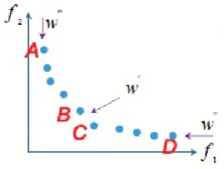
assign a weight to each objective function and search in one direction. But, this approach has some shortcomings; for example, as seen in Figure 1, with a weight vector asw0 = (0.5,0.5)forf1andf2objective functions, it is possible to findBandCPareto optimal solutions easily but findingAandDpoints is difficult [10][31].
Figure 1.The multiple weight vector approach
The multiple weight vector can be applied to overcome this deficiency, because in this case, the search is done in different directions. There are many methods to apply this approach in the literature, (i) the Schaffer’s method, in which, the population is divided intoM sub-populations, then it is adapted toMfitness functions asf1(x), f2(x), ..., fM(x)[37]; (ii) the Kursawe’s
method that is similar to the Schaffer’s method, while a probability is assigned to each objective function to choose a specific direction to search on it [23][30] and (iii) the Ishibuchi and Murata’s method, in which weights of the objective functions are selected randomly [31].
The posterior approach is generally more preferred, where, the preference information of decision maker is not known in advance and the appropriate solutions are selected from the obtained ones after the search. In this approach, the Pareto optimality and the domination concepts are used. Solution S1 dominates solutionS2 (denoted as S1 S2), if and only if (∀i∈M :fi(S1)≤fi(S2))f(∃i∈M :fi(S1)< fi(S2))andS1is a Pareto optimal solution, if and only if¬∃S2:S2S1.
If setPas contains all of the Pareto optimal solutions asPas = {S1|¬∃S2 : S2 S1}that is the Pareto front. The set of
corresponding values of the objective functions inPas as PF = {f(s) = (f0(s), f1(s), ..., fm−1(as))|z ∈ Pas}is the set of Pareto optimal front. IfPas is infinite, it is difficult to find it with finite solutions, so a subset of the set can be desired. The
intended subset must be a good estimation of the Pareto front with a good diversity [10][21][51].
There are many evolutionary algorithms in the literature based on the Pareto optimality concept. The non-dominated sorting genetic algorithm (NSGA) and the NSGA-II are between the most famous of them based on the Pareto optimality concept. The NSGA that is presented by Deb and Srinivas has some shortcomings as (i) thehigh complexity, of the non-dominated sorting, which isO(mN3)at each iteration, (ii) thelack of elitismand (iii) thediversity adjustment requirement[13][15][35][54].
The NSGA-III algorithm, proposed by Deb and Jian in 2014, is similar to the NSGA-II but uses different selection operators. It begins with determining the reference points (H) to place on the hyperplane. This also provides the diversity of the obtained solutions. This reference-point-based many-objective algorithm emphasizes population members that are non-dominated, yet close to a set of supplied reference points. The many-objective optimization problems contain four or more objectives. Two-objective and three-Two-objective problems fall into a different class as the resulting Pareto-optimal front. Mostly, they can be comprehensively visualized by graphical means. But a strict upper bound on the number of objectives for a many-objective optimization problem is not so clear, except for a few occasions, most practitioners are interested in a maximum of 10–15 objectives. Ciro et al., have compared the NSGA-II and NSGA-III algorithms for solving an open shop scheduling problem with resource constraints to minimize the total flow time and balancing the resources workload. Both of them have a similar performance, however, the NSGA-III has a slight higher hyper-volume average than the NSGA-II. In addition, the NSGA-III has better results for the large-sized benchmarks and also for those that have more than 2 objectives. This is because of the process of defining a hyperplane and some reference points to classify the solutions and also for selecting the best qualified for the next population [9][14][32].
front. The comparison performs according to the non-dominated rank (irank) and the local crowding distance (idistance), whose
complexity isO(2Nlog(2N)).
Several metrics are used for quantifying the performance of the multi-objective evolutionary algorithms. For example, there are some criteria to measure theaccuracy, thecoverageand thevariance. The accuracy shows the closeness between the genera-ted non-dominagenera-ted and the best known solutions. The coverage indicates the diversity of solutions, while the variance represents the maximum range covered by a solution in the non-dominated front. There are various metrics in the literature to measure the diversity. The front spread (FS) that is proposed by Zitzler, is a suitable indicator of the diversity. The large values of this metric are desired [53]. In addition to the diversity, it is important to know that how many points are in the non-dominated solutions set. The front occupation (FO) is a measure suggested by Van Veldhuizen, which is defined in Equation 4 and its large values are desired [53].
F O=|F1| (4)
|F1|is the number of solutions on the Pareto front. Dis another measure proposed by Van Veldhuizen whose small values are desired. This measure that is defined in Equation 5, can’t properly represent the diversity because it indicates the average distance between the achieved solutions from the Pareto front [53].
D= 1
|F1|
X
S
d(S1, S2) (5)
d(S1, S2)are the distance between solutionsS1andS2according to the objective functions (fi) in the Euclidean distance
system, which are calculated as Equation 6 [53], wheremis the number of objectives.
d(S1, S2) =
v u u t
m−1
X
i=0
(fi(S2)−fi(S1))2 (6)
In the NSGA-II, theMmeasure is used to evaluate the distribution of the points in the first front of the Pareto solutions. This measure is defined as Equation 7 [13][15].
M=
|F1|
X
i=1
|di−d¯|
|F1| (7)
diis the distance between two successive solutions in the Pareto front as it is defined in Equation 6 andd¯is the average of
them, which is calculated for the last iteration. After 10 iterations, the average and variance of theMare calculated for compari-son [13][15].
Tavakkoli et al. have designed an algorithm, which is compared with the NSGA-II, according to (i) a quality metric, (ii) a spacing metric and (iii) a diversification metric. Non-dominated solutions of the algorithms are put together and their ratio is calculated with the quality metric. Spacing metric that is defined as Equation 8, measures the uniformity of the solutions [40].
SP C =
P|F1|−1
i=1 |d¯−di|
(|F1| −1)×d¯ (8)
Construction of the Pareto fronts in the MO-JSSP needs high computational effort, especially in the large-size problems, which have more than 20 jobs and 10 machines. So, achieving the Pareto front in a short time and with a small memory demon-strates the efficiency of the algorithm. Suresh and Mohanasundaram have reported that they have achieved a good solution set in a short computational time and with a small memory [38]. They have used thenet front contribution ratio(NFCR) metric to measure the quality of the non-dominated solution set [29]. NFCR is a relative measure that uses thenet non-dominated frontas thereference set. The net non-dominated front is obtained by updating the combined non-dominated front, which consists of the all non-dominated solutions of the compared algorithms. Fistands for the non-dominated front of thei-th algorithm, whileFn
is the front of all algorithms. ni andnnare respectively the numbers of solutions in the non-dominated individuals of thei-th
algorithm and the net front (Fn). For each of the compared algorithm, the net front contribution ratio is calculated according to
N F CRi=
ni
nn
(9)
4
Algorithm and Implementation
[image:6.595.141.459.198.622.2]The general steps of the NSGA-II algorithm are summarized in Figure 2, which are similar to the M1-NSGA-II and M2-NSGA-II.
Figure 2.Flowchart of the NSGA-II
In the NSGA-II, the initial population is generated randomly, while in the M1-NSGA-II and M2-NSGA-II, 84%of the initial population is generated by the Giffler and Thompson (GT) algorithm [43] and the remainder part is created randomly. Each solution is expressed as a chromosome, which consists of two parts. As seen in Figure 3, the first part represents the order of operations, while the second part shows the assigned machines.
Figure 3.A chromosome that consists of two parts to represent the order of operations and the assigned machines
[image:6.595.132.462.693.728.2]are selected through the tournament selection. For this purpose, if a solution is dominated, it is eliminated. If none of them is dominated by the other, the one with the better crowding distance is chosen as the parent. Crossover is defined as a one-point operator that is applied to the first part. The mutation is done with a constraint-based neural network that creates feasible neighbors. It applies penalties to infeasible neighbors and transforms them to feasible ones. In this way, during the mutation, a feasible neighbor is generated for the selected individuals, according to the structures summarized in Algorithm 3.
Algorithm 1: Non-dominated sorting
1 Input: Population (P); 2 Output: FrontsFi; 3 S←P;
4 whileS6=φdo
5 i= 1;
6 foreachp∈Sdo
7 Sp=φ(The set of solutions thatpdominates them); 8 np= 0(The number of solutions that dominatep);
9 foreachq∈Sdo
10 ifp≺qthen
11 Sp=Sp∪q;
12 else ifq≺pthen
13 np=np+ 1;
14 end
15 end
16 ifnp= 0then
17 Fi=Fi∪p;
18 end
19 end
20 ExcludepfromS;
21 ifFi=φthen
22 Exit;
23 else
24 i=i+1;
25 end
26 end
Algorithm 2: Calculate crowding distances
1 Input: FrontsFi;
2 Output: Crowding distances (dsij: crowding distance for solutionjon fronti); 3 foreachFront (Fi)do
4 foreachObjective function (m)do
5 Sortsolutions onFiaccording to objectivem;
6 Findboundary solutionssmi1andsmil and assign a big value to their crowding distances;
7 (dms
i1andd
m
sil← ∞);
8 forj= 2; j < l−1; j=j+ 1do
9 dsij =dsij +
dm si(j+1)−d
m si(j−1)
dm
max−dmmin ;
10 end
11 end
Figure 4.Crowding distance between to solutions
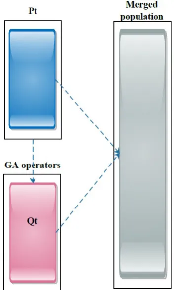
As seen in Figure 5, in the NSGA-II, theQtis merged with the parent population (Pt).
Figure 5.The creation of the merged population in the NSGA-II
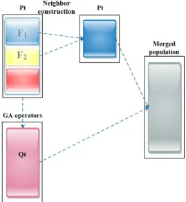
In the M1-NSGA-II, as shown in Figure 6, after that theQtis generated using the crossover and mutation operators, a
neig-hbor is constructed for each individual using a neigneig-hborhood structure selected randomly from the structures that are summarized in Algorithm 3. If the neighbor dominates the parent, it is replaced with the parent. Else if the parent dominates the neighbor it reminds in the population. If they do not dominate the other, one of them is selected randomly, then theQtis merged with the
[image:8.595.210.387.370.664.2]Figure 6.The construction of the merged population in the M1-NSGA-II
As seen in Figure 7, in the M2-NSGA-II, after creation of theQtusing the crossover and mutation operators, a neighbor is
created only for the solutions on the first and second fronts of thePt, using a neighborhood structure selected randomly from
Algorithm 3. Then they are merged with theQt.
[image:9.595.162.432.466.759.2]The used neighborhood structures are summarized in Algorithm 3.
Algorithm 3: Neighborhood structures
1 Input: Solution; 2 Output: Neighbor; 3 ifi==1then
4 Swap the operations on the same critical blocks; 5 else ifi==2then
6 Swap the operations of the critical path which are on different machines; 7 end
8 else ifi==3then
9 Insert the operations on the critical path to the different positions; 10 end
11 else ifi==4then
12 Swap the operations on the critical blocks with the first operation of the same critical block; 13 end
14 else ifi==5then
15 Swap the operations on the critical blocks with the last operation of the same critical block; 16 end
17 else ifi==6then
18 Swap the first and the last operations of the blocks; 19 end
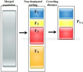
In the all algorithms, the merged population is sorted using the non-dominated sorting and crowding distances, then the new population (Pt+1) is created with selecting solutions as much as the population size. These processes are summarized in Figure
[image:10.595.151.442.414.666.2]8.
Figure 8.New population generation in the algorithms
5
Results and Comparison
Table 2.Parameters of the proposed M-NSGA-II
Parameter Value
Population size 50
Crossover rate 100%
Mutation rate 20%
Number of iterations 100
The MK01 from the BRData instances is used as the benchmark, whose best intervals in literature are summarized in Table 3 [25].
Table 3.Best intervals of the objective functions in the literature for the MK01 instance [25] (NS: Number of non-dominated solutions in the literature)
Cmax Wm WT NS
(40,45) (36,42) (153,169) 11
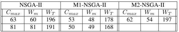
[image:11.595.149.443.417.470.2]The described algorithms are implemented in MATLAB 2017b on a system with a Core i7 6700HQ processor and 32 GB RAM. The obtained results are summarized in Table 4. The NSGA-II, M1-NSGA-II and M2-NSGA-II have found 2, 2 and 1 Pareto solutions, respectively. The order of operations and the assigned machines in these solutions are presented in the appendix.
Table 4.The obtained results
NSGA-II M1-NSGA-II M2-NSGA-II
Cmax Wm WT Cmax Wm WT Cmax Wm WT
63 60 196 53 48 178 62 54 197
81 81 191 50 49 168
[image:11.595.182.408.591.631.2]The comparison between the algorithms based on the measuresFOandNFCR, defined in Equations 4 and 9, is summarized in Table 5. The solutions achieved by the M1-NSGA-II dominate the other ones obtained by the NSGA-II and M2-NSGA-II algorithms. Therefore, itsNFCRvalue is equal to 1. None of the solutions obtained by the other 2 algorithms dominate the others, so theirNFCRvalues are equal to 0.
Table 5.The comparison based on the measuresFOandNFCR
NSGA-II M1-NSGA-II M2-NSGA-II
FO 2 2 1
NFCR 0 1 0
6
Conclusion and Future Works
when heuristics such as the Giffler and Thompson algorithm and the local left shifts are used for initial solutions creation, and even to improve the solutions during the iterations. Based on the results obtained from the M2-NSGA-II, we can make another conclusion that it is better to define that the neighborhood structures should be applied to how many solutions and which ones. Otherwise, the performance of the algorithm may not improve.
In future work, we plan to design a multi-objective particle swarm optimization (MO-PSO) algorithm for solving scheduling problems.
REFERENCES
[1] O. Bahadir, G. Ozturk, and A. Teymourifar. Extracting new dispatching rules for dynamic multi-objective scheduling problems using simulation and gep. In3 rd INTERNATIONAL RESEARCHERS, STATISTICIANS AND YOUNG STATIS-TICIANS CONGRESS 24-26 MAY 2017 SELÇUK UNIVERSITY, 2017.
[2] J. Behnamian, M. Zandieh, and S. F. Ghomi. Parallel-machine scheduling problems with sequence-dependent setup times using an aco, sa and vns hybrid algorithm.Expert Systems with Applications, 36(6):9637–9644, 2009.
[3] D. Behnke and M. J. Geiger. Test instances for the flexible job shop scheduling problem with work centers. https:
//www.deutsche-digitale-bibliothek.de/item/WG35B3KZZC4YAARHH3GSHGXEKWRZHY5L.
[4] D. Behnke and M. J. Geiger. Test instances for the flexible job shop scheduling problem with work centers. 2012.
[5] J. H. Blackstone, D. T. Phillips, and G. L. Hogg. A state-of-the-art survey of dispatching rules for manufacturing job shop operations. The International Journal of Production Research, 20(1):27–45, 1982.
[6] J. Bła˙zewicz, W. Domschke, and E. Pesch. The job shop scheduling problem: Conventional and new solution techniques. European journal of operational research, 93(1):1–33, 1996.
[7] P. Brandimarte. Routing and scheduling in a flexible job shop by tabu search. Annals of Operations research, 41(3):157– 183, 1993.
[8] J. B. Chambers and J. W. Barnes. Tabu search for the flexible-routing job shop problem. Graduate program in Operations Research and Industrial Engineering, The University of Texas at Austin, Technical Report Series, ORP96-10, 1996.
[9] G. C. Ciro, F. Dugardin, F. Yalaoui, and R. Kelly. A nsga-ii and nsga-iii comparison for solving an open shop scheduling problem with resource constraints.IFAC-PapersOnLine, 49(12):1272–1277, 2016.
[10] C. A. C. Coello, G. B. Lamont, D. A. Van Veldhuizen, et al.Evolutionary algorithms for solving multi-objective problems, volume 5. Springer, 2007.
[11] S. Dauzère-Pérès and J. Paulli. Solving the general multiprocessor job-shop scheduling problem.Working Papers, Depart-ment of Mathematical Sciences, University of Aarhus, 1995.
[12] S. Dauzère-Pérès and J. Paulli. An integrated approach for modeling and solving the general multiprocessor job-shop scheduling problem using tabu search. Annals of Operations Research, 70:281–306, 1997.
[13] K. Deb, S. Agrawal, A. Pratap, and T. Meyarivan. A fast elitist non-dominated sorting genetic algorithm for multi-objective optimization: Nsga-ii. InParallel problem solving from nature PPSN VI, pages 849–858. Springer, 2000.
[14] K. Deb and H. Jain. An evolutionary many-objective optimization algorithm using reference-point-based nondominated sorting approach, part i: Solving problems with box constraints. IEEE Trans. Evolutionary Computation, 18(4):577–601, 2014.
[15] K. Deb, A. Pratap, S. Agarwal, and T. Meyarivan. A fast and elitist multiobjective genetic algorithm: Nsga-ii.Evolutionary Computation, IEEE Transactions on, 6(2):182–197, 2002.
[16] M. Dell’Amico and M. Trubian. Applying tabu search to the job-shop scheduling problem.Annals of Operations Research, 41(3):231–252, 1993.
[17] P. Fattahi, M. S. Mehrabad, and F. Jolai. Mathematical modeling and heuristic approaches to flexible job shop scheduling problems. Journal of Intelligent Manufacturing, 18(3):331–342, 2007.
[19] N. B. Ho, J. C. Tay, and E. M.-K. Lai. An effective architecture for learning and evolving flexible job-shop schedules. European Journal of Operational Research, 179(2):316–333, 2007.
[20] O. Holthaus and C. Rajendran. Efficient dispatching rules for scheduling in a job shop.International Journal of Production Economics, 48(1):87–105, 1997.
[21] T. Hsu, R. Dupas, D. Jolly, and G. Goncalves. Evaluation of mutation heuristics for solving a multiobjective flexible job shop by an evolutionary algorithm. InSystems, Man and Cybernetics, 2002 IEEE International Conference on, volume 5, pages 6–pp. IEEE, 2002.
[22] J. Hurink, B. Jurisch, and M. Thole. Tabu search for the job-shop scheduling problem with multi-purpose machines. Operations-Research-Spektrum, 15(4):205–215, 1994.
[23] H. Ishibuchi and T. Murata. A multi-objective genetic local search algorithm and its application to flowshop scheduling. Systems, Man, and Cybernetics, Part C: Applications and Reviews, IEEE Transactions on, 28(3):392–403, 1998.
[24] H. Ishibuchi, T. Yoshida, and T. Murata. Balance between genetic search and local search in memetic algorithms for multiobjective permutation flowshop scheduling. IEEE transactions on evolutionary computation, 7(2):204–223, 2003. [25] S. Jia and Z.-H. Hu. Path-relinking tabu search for the multi-objective flexible job shop scheduling problem.Computers &
Operations Research, 47:11–26, 2014.
[26] I. Kacem, S. Hammadi, and P. Borne. Approach by localization and multiobjective evolutionary optimization for flexible job-shop scheduling problems. Systems, Man, and Cybernetics, Part C: Applications and Reviews, IEEE Transactions on, 32(1):1–13, 2002.
[27] I. Kacem, S. Hammadi, and P. Borne. Pareto-optimality approach for flexible job-shop scheduling problems: hybridization of evolutionary algorithms and fuzzy logic. Mathematics and computers in simulation, 60(3):245–276, 2002.
[28] J. Knowles and D. Corne. The pareto archived evolution strategy: A new baseline algorithm for pareto multiobjective optimisation. InEvolutionary Computation, 1999. CEC 99. Proceedings of the 1999 Congress on, volume 1, pages 98–105. IEEE, 1999.
[29] J. D. Knowles.Local-search and hybrid evolutionary algorithms for Pareto optimization. PhD thesis, Department of Com-puter Science Local-Search and Hybrid Evolutionary Algorithms for Pareto OptimiZation Joshua D. Knowles Submitted in partial fulfilment of the requirements for the degree of Doctor of Philosophy in Computer Science. Department of Computer Science, University of Reading, 2002.
[30] F. Kursawe. A variant of evolution strategies for vector optimization. InParallel Problem Solving from Nature, pages 193–197. Springer, 1990.
[31] Y.-W. Leung and Y. Wang. Multiobjective programming using uniform design and genetic algorithm. Systems, Man, and Cybernetics, Part C: Applications and Reviews, IEEE Transactions on, 30(3):293–304, 2000.
[32] H. Nakayama, K. Kaneshige, S. Takemoto, and Y. Watada. An application of a multi-objective programming technique to construction accuracy control of cable-stayed bridges.European Journal of Operational Research, 87(3):731–738, 1995. [33] E. Nowicki and C. Smutnicki. A fast taboo search algorithm for the job shop problem.Management science, 42(6):797–813,
1996.
[34] V. Roshanaei, B. Naderi, F. Jolai, and M. Khalili. A variable neighborhood search for job shop scheduling with set-up times to minimize makespan.Future Generation Computer Systems, 25(6):654–661, 2009.
[35] G. Rudolph. Evolutionary search under partially ordered sets. Dept. Comput. Sci./LS11, Univ. Dortmund, Dortmund, Germany, Tech. Rep. CI-67/99, 1999.
[36] C. Santos, J. Spim, and A. Garcia. Mathematical modeling and optimization strategies (genetic algorithm and knowledge base) applied to the continuous casting of steel. Engineering Applications of Artificial Intelligence, 16(5):511–527, 2003. [37] J. Schafer. Multi-objective optimization with vector evaluated genetic algorithm. InProceedings of the 1st International
Conference on Genetic Algorithms, pages 93–100.
[39] E.-G. Talbi.Metaheuristics: from design to implementation, volume 74. John Wiley & Sons, 2009.
[40] R. Tavakkoli-Moghaddam, M. Azarkish, and A. Sadeghnejad-Barkousaraie. A new hybrid multi-objective pareto archive pso algorithm for a bi-objective job shop scheduling problem.Expert Systems with Applications, 38(9):10812–10821, 2011. [41] A. Temourifar and G. Ozturk. New dispatching rules and due date assignment models for job shop scheduling problems.
Accepted to International Journal of Manufacturing Research, 2017.
[42] A. Teymourifar and G. Ozturk. A hybrid pareto-based swarm optimization algorithm for the multi-objective flexible job shop scheduling problems. World Academy of Science, Engineering and Technology, International Journal of Mechanical and Industrial Engineering, 4(7), 2017.
[43] A. Teymourifar and G. Ozturk. A neural network-based hybrid method to generate feasible neighbors for flexible job shop scheduling problem. Universal Journal of Applied Mathematics, 6(1):1–16, 2018.
[44] A. Teymourifar, G. Ozturk, and O. Bahadir. A constrained neural network based variable neighborhood search for the multi-objective dynamic flexible job shop scheduling problems. World Academy of Science, Engineering and Technology, International Journal of Mechanical and Industrial Engineering, 4(7), 2017.
[45] B.-O. Teymourifar, Aydin and G. Ozturk. Dynamic priority rule selection for solving multi-objective job shop scheduling problems. Universal Journal of Industrial and Business Management, 6(1):11–22, 2018.
[46] L.-F. Tung, L. Lin, and R. Nagi. Multiple-objective scheduling for the hierarchical control of flexible manufacturing systems. International Journal of Flexible Manufacturing Systems, 11(4):379–409, 1999.
[47] P. Vachhani, R. Rengaswamy, and V. Venkatasubramanian. A framework for integrating diagnostic knowledge with non-linear optimization for data reconciliation and parameter estimation in dynamic systems. Chemical Engineering Science, 56(6):2133–2148, 2001.
[48] W. Xia and Z. Wu. An effective hybrid optimization approach for multi-objective flexible job-shop scheduling problems. Computers & Industrial Engineering, 48(2):409–425, 2005.
[49] L.-N. Xing, Y.-W. Chen, P. Wang, Q.-S. Zhao, and J. Xiong. A knowledge-based ant colony optimization for flexible job shop scheduling problems.Applied Soft Computing, 10(3):888–896, 2010.
[50] L.-N. Xing, Y.-W. Chen, and K.-W. Yang. An efficient search method for multi-objective flexible job shop scheduling problems. Journal of Intelligent Manufacturing, 20(3):283–293, 2009.
[51] Y. Yuan and H. Xu. Multiobjective flexible job shop scheduling using memetic algorithms. Automation Science and Engineering, IEEE Transactions on, 12(1):336–353, 2015.
[52] G. Zhang, X. Shao, P. Li, and L. Gao. An effective hybrid particle swarm optimization algorithm for multi-objective flexible job-shop scheduling problem. Computers & Industrial Engineering, 56(4):1309–1318, 2009.
[53] E. Zitzler.Evolutionary algorithms for multiobjective optimization: Methods and applications, volume 63. Citeseer, 1999. [54] E. Zitzler, K. Deb, and L. Thiele. Comparison of multiobjective evolutionary algorithms: Empirical results. Evolutionary
Appendices
The achieved solutions by the NSGA-II (S1,S2), the M1-NSGA-II (S3,S4) and the M2-NSGA-II (S5) are as follows: