A multi factor decomposing model and its application in finding impacting factors of Beijing water use efficiency

(1)

Journal of Chemical and Pharmaceutical Research, 2013, 5(12):543-547

Research Article

_{CODEN(USA) : JCPRC5}

ISSN : 0975-7384

A multi-factor decomposing model and its application in finding impacting

factors of Beijing water use efficiency

1

**X. L. Liu*,**

2

G. J. D. Hewings,

1

X. K. Chen and

1

SH. Y. Wang

1

Academy of Mathematics and Systems Science, Chinese Academy of Sciences, Zhongguancun

East Road No.55, Beijing, China

2

Regional Economics Applications Laboratory, University of Illinois, 607 S. Mathews, #318,

Urbana, IL, USA

____________________________________________________________________________________________

ABSTRACT

The main purpose of this study was to explore factors affecting water use efficiency (WUE) by sector and find ways to improve it. A new Multi-Sector and Multi-Factors Logarithmic Mean Divisia Index (MLMDI) decomposing model was established in the paper. The model can decompose the change of WUE by sector into 14 factors definitely which can reveal 10 kinds of technology and structure effects and include indirect impacts. Applied the MLMDI model to Beijing, the affecting extent of 14 factors on WUE of 19 sectors during 2002-2007 were figured out. It was found that during 2002-2007 the drop of export and transfer out ratio of agriculture, the increase of grain production by unit of arable area had evident effects on improving water use efficiency by each sector. Industrial structure adjustment and labor structure change among different sectors had small impact on improving water use efficiency.

Keywords: Multi-factor decomposing model, Water use efficiency, Input- output analysis, Beijing

____________________________________________________________________________________________

INTRODUCTION

As the competition for the finite water resources on earth increases due to growth in population and affluence, industries are faced with intensifying pressure to improve the efficiency of water use. The efficiency of water use can be improved further through technological innovations, new policies and simple improvements in operations. In the 1930s and 1940s, steel production for example typically consumed up to 200-300 tones of water per ton of steel.

Today just 3-4 tons of water is required to do the same job in the most efficient plants [1]. More and more water

suppliers and planning agencies are beginning to explore efficiency improvements to lessen pressures on increasingly scarce water resources, reduce the adverse ecological effects of human withdrawals of water, and improve long-term sustainable water use [2-5].

The causes for the relatively low water use efficiency by different sector are numerous and complex, including environmental, management, engineering, social and economic facets. The complexity of the problem, with its myriads of local variations, requires a comprehensive conceptual framework as the basis to analyze the existing situation and quantify the efficiencies, and to plan and execute improvements.

(2)

quantify water use efficiency. Within this framework, [7] studied the supply and demand balance for water resources in Shanxi Province of China. [8] developed a hydro economic model by incorporating the water industries into the input-output table. [9] evaluated the internal effect and the induced effect of water use efficiency in Spain. [10] established a number of indicators to evaluate water use efficiency and study the intersectoral water relationships in the economy of Andalusia. [11] provided an improved index to evaluate water use efficiency by incorporating fixed assets effects.

To find the affecting factors of water use efficiency, decomposing analysis will be applied. There are two broad categories of decomposition techniques: structural decomposition analysis (SDA) and index decomposition analysis (IDA) [12]. One advantage of SDA is that the input-output model includes indirect demand effects–demand for inputs from supplying sectors that can be attributed to the downstream sector’s demand. So that SDA can differentiate between direct and indirect demands. While the IDA model is incapable of capturing indirect demand effects before this research. There are several different SDA decomposition forms to the same variable. Many researches [13-19] made great contributions to the design and the improvement of the SDA method. Thanks to the greater structural details in the input-output table, SDA has another advantage of being able to distinguish between a range of technological effects and structural effects. While SDA has some drawbacks in data limitation for I-O table is often dray up every five years. IDA can be applied to any available data at any level of aggregation. It is more widely used owing to not high demand for data and is easily handled with time series and pool data.

There are a variety of different indexing methods that can be used in IDA ([16], [20]). Several variants of the IDA approach have been developed [21-23]. However, to a large extent, selection of method seems to be arbitrary and there is little consensus as to which one is the superior method. [16] and [23-24] argued that the logarithmic mean divisia index (LMDI) method should be preferred to other decomposition methods with the advantages of path independency, ability to handle zero values and consistency in aggregation. While to the literatures concerned with LMDI models we have ever reviewed, they usually decomposed one index into 3-5 affecting factors like technological effect and structure effect. These factors were covering a wide range of meaning, which were difficult to be tracked and adjusted in practice. To relax the limitations of the LMDI model, this paper provided a new decomposing analysis model (MLMDI) with the aid of input-output analysis. The paper is organized as follows. Section 2 presents MLMDI model. Section 3 describes dataset. Section 4 applies the model and presents the calculation results. Section 6 gives conclusions.

MLMDI MODEL

The paper compiled 2002 and 2007 Beijing water resource IOO tables with the framework in [11]. The total water

use coefficient

I

w

t

was applied to evaluated water use efficiency. It was defined as [11],

(

₋ ₋_ˆ

)

−1

=Iwd I A D t

w

I γ (1)

where D represents the direct occupancy coefficients matrix of fixed assets.

γ

ˆ

is a diagonal matrix of fixed assets

depreciation rate.

j j

j Iwt y

wt = * (2)

where j

y is the final consumption of sector j.wtjmeans the amount of water used directly and indirectly to

produce

j

y .

In equation (2), for _>₀

j

t w

I , ifyj<0, it will bewtj<0. It means,wtj/yj=wtj /yj (3)

From equations (2) and (3), equation (4) can be deduced.

j j n j j j j j j j

j wt y wt y wd wd wt wd

t w

I / / / * /

1

∑

= = = = *

_∑

= = n j n j j j Va wd 1 1

/ * n _j

j j Va Va / 1

∑

= * j j L

Va / *

_∑

= n j j j L L 1

/ * L RP

n j j/ 1

∑

=

*RP /AA*AA/GP*

1 / wd

GP *wd1/ Ex1*

∑

= n j j Ex Ex 1 1/ * j n j j Ex Ex / 1

∑

= * j j y

Ex / (4)

where

j

Va is the value added of sector j, L is the number of employees by sector j. RP is the size of rural _j

population, AA is the arable land area, GP is grain production volume in the research year,

1

wd is the volume of

water used directly by sector 1,

j

(3)

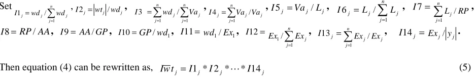
Set

∑

= = n j j j j wd wd

I

1

/

1 ,I2j=wtj/wdj,

∑

= = = n j n j j j Va wd I 1 1 /

3 ,

∑

= = n

j j j j Va Va

I

1 /

4 ,I5j =Vaj/Lj,

∑

=

= n

j j j

j L L

I

1

/

6 , I7=

_∑

= n j j RP L 1 / , = 8

I RP /AA, I9= AA /GP, I10=GP/ wd₁, I11=wd₁/ Ex₁, I12=

_∑

= n j j Ex Ex 1 1/ , ₌ j I13 j n j j Ex Ex / 1

∑

=

, I14_j ₌Ex /_j y_j .

Then equation (4) can be rewritten as,

j j

j

j I I I

t w

I = 1 * 2 *L* 14 (5)

It means _I_w_t_jcan be decomposed into 14 factors. The economic meaning of them and the technology and structure

they represented were clear.

The change of total water use coefficient by sector j (_∆_I_w_t_j) from time 0 to time 1 can be decomposed as follows.

j t w I

∆ = 1 0

j j Iwt

t w

I − = 1 1 1

14 * * 2 *

1_j I _j I _j

I L - ₁0_* ₂0_* _* ₁₄0

j j

j I I

I L

= I1

j

t w I

∆ + I2

j

t w I

∆ +…+ I14

j

t w I

∆ + rsd

j t w I

∆ (6)

Set ( 1 0)/ln( 1/ 0)

j j j

j

j Iwt Iwt Iwt Iwt

L = − (7)

Then: Ik

j

t w I

∆ =L_j*ln(Ik1_j/Ik0_j) (j=1, 2…n; k=1, 2…14) (8)

j

t

w

I

∆

=

_∑

= ∆ 14 1 k Ik j t w

I (j=1, 2…n) (9)

rsd j t w I

∆ =0 (j=1, 2…n) (10)

DATA SOURCE

In the paper, Water Resource IOO tables of Beijing in 2002 and 2007 were compiled. The input-output tables with 42 sectors published by Beijing Statistics Bureau were aggregated to form tables with 19 sectors (See Appendix A) for water data limitation, which highlighted water-intensive sectors 1-10 [25].The direct water use data for 4 main sectors (agriculture, industry, domestic and environment) sourced from Beijing Water Bulletin 2002 and 2007. The detailed direct water use data by industrial sectors were deduced from [25] and [26] and Beijing Water Bulletin 2002 and 2007. The detailed direct water use data by tertiary industries were deduced from [27] and Beijing Water Bulletin 2002 and 2007. The employees and the fixed assets data was cited from Beijing Statistics Book 2003, 2008 and Beijing Economic Survey 2008.

RESULTS

With

I

w

t

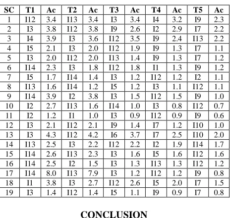
as an index to evaluate water use efficiency, applied MLMDI model, ∆Iwt_j(j=1, 2…19) of Beijing from

2002 to 2007 can be decomposed into 15 parts separately. Results see Table 1(Only top 5 factors were listed).

Table 1 showed that, (1) For all sectors, I3 and I12 almost fell in top 5 impact factors, IF9 ranked in the top 3-8 affecting factors. These showed that reducing the direct water use by unit value added had evident effect on improving water use efficiency, which is very evidently but this verified the rationality of the model. More important, these told us that lower the export and transfer out ratio of agriculture, increase the grain production by unit of arable area had evident effects on improving water use efficiency by each sector.

(2) I4 was the top 1 impact factor to sector 3, the top 4 impact factor to sector 1, the top 7 impact factor to sector 6, sector 10 and sector 16. To the other 14 sectors, I4 was ranked in the last 4 impact factor. These revealed that adjust

industrial structure was not the best way to reduce Iwt_jof most sectors during 2002-2007. [28] indicated that

industrial structure adjustment presented the rising trend of the contribution rate of water saving during 1990-2000 years, the contribution was 29.5% during 1990-1994, while it was 46.1% during 1998-2000. After 2000, there was little water saving potential by industrial structure adjustment.

[image:3.595.73.541.75.151.2]

(4)

[image:4.595.191.423.137.357.2]

(4) To all sectors, I8 ranked in the last 5 impact factor. I7 fell in the top 4-9 impact factor, which showed that control the process of urbanization at a rational speed was conducive to water conservation.

Table 1: The top 5 factors of ∆Iwt_j(j=1,2...19) and their contributions Ac ( Ik j

Ac = Ik

j t w I

∆ /

j

t w I

∆ )

SC T1 Ac T2 Ac T3 Ac T4 Ac T5 Ac

1 I12 3.4 I13 3.4 I3 3.4 I4 3.2 I9 2.3 2 I3 3.8 I12 3.8 I9 2.6 I2 2.9 I7 2.2 3 I4 3.9 I3 3.6 I12 3.5 I9 2.4 I13 2.2 4 I5 2.1 I3 2.0 I12 1.9 I9 1.3 I7 1.1 5 I3 2.0 I12 2.0 I13 1.4 I9 1.3 I7 1.2 6 I14 2.3 I3 1.8 I12 1.8 I1 1.3 I9 1.2 7 I5 1.7 I14 1.4 I3 1.2 I12 1.2 I2 1.1 8 I13 1.6 I14 1.2 I5 1.2 I3 1.1 I12 1.1 9 I14 3.9 I2 3.8 I3 1.5 I12 1.5 I9 1.0 10 I2 2.7 I13 1.6 I14 1.0 I3 0.8 I12 0.7 11 I2 1.2 I1 1.0 I3 0.9 I12 0.9 I9 0.6 12 I3 2.1 I12 2.1 I9 1.4 I7 1.2 I10 1.0 13 I3 4.3 I12 4.2 I6 3.7 I7 2.5 I10 2.0 14 I13 2.5 I3 2.2 I12 2.2 I2 1.9 I14 1.7 15 I14 2.6 I13 2.3 I3 1.6 I5 1.6 I12 1.6 16 I14 2.5 I2 1.5 I3 1.3 I13 1.3 I12 1.2 17 I14 8.0 I13 7.9 I3 1.2 I12 1.2 I9 0.8 18 I1 3.8 I3 2.7 I12 2.6 I5 2.0 I7 1.5 19 I3 1.4 I12 1.4 I5 1.1 I9 0.9 I7 0.8

CONCLUSION

The paper established a new MLMDI decomposing model. Not like the existed LMDI models, this model is capable of capturing indirect demand effects. It can decompose one index into 14 elements definitely by sector which can reveal 10 kinds of technological and structure effects like economic structure, labor structure, urban and rural structure, export and transfer out structure, direct water use structure, water use multiplier, productivity of labor, water use intensity of agriculture et al. It is more capable to distinguish between a range of technological effects and structural effects than SDA method. Furthermore, most of these decomposing factors are easily to be tracked and adjusted in practice. This modeling framework can be extended to make energy, land and other natural resources use efficiency decomposition analysis in different regions.

Applied the model to Beijing, it is found that, during 2002-2007 the drop of export and transfer out ratio of agriculture, the increase of grain production by unit of arable area had evident effects on improving water use efficiency by each sector. Industrial structure adjustment and labor structure change among different sectors had small impact on improving water use efficiency.

Acknowledgements

We would like to acknowledge the support from the National Natural Science Foundation of China (No.70701034, No.71173210 and No.61273208). We appreciate the anonymous reviewers for their helpful comments and suggestions on the paper.

REFERENCES

[1] PH Gleick; Nature, 2002, 418(25), 373.

[2] J Xia; Water International, 2010, 35(3), 247-249.

[3] W Chen, SHJ Zhu; MY Lai; 2010 International Conference on Management Science& Engineering (17th), 2010, Nov. 24-26, Melbourne, Australia.

[4] PH Gleick;Water International, 2000, 25(1), 127-138.

[5] PH Gleick; Annual Review of Environment and Resources, 2003, 28, 275-314.

[6] EM Lofting; PH McGauhey. Economic valuation of water. An Input-Output Analysis of California Water Requirements, Contribution 116. University of California Water Resources Center, Berkeley, 1968; 42-53.

[7] X Chen; Thirteenth International Conference on Input-Output Techniques, 2000, August 21-25, Macerata, Italy. [8] H Bouhia.Water in the Macroeconomy: Integrating Economics and Engineering into an Analytical Model. Aldershot, Ashgate Publishing Limited, UK, 2001; 86-92.

[9] R Duarte; JS Cho′ liz; J Bielsa; Ecological Economics, 2002,43(2), 71-85.

(5)

[11] XL Liu; Journal of Water Resource and Protection, 2012, 4(5), 264-276. [12] R Hoekstra; JCJM Van der Bergh; Energy Economics, 2003, 25(1), 39-64.

[13] L Shapley. A value for n-person games. In: Kuhn H.W., Tucker A.W. (Eds), Contributions to the theory of games, Princeton University: Princeton, 2, 1953; 307-317.

[14] A Rose; S Casler; Economic Systems Research, 1996, 8(1), 33-62. [15] BW Ang; KH Choi; The Energy Journal, 1997, 18(3), 59-73. [16] BW Ang; F Q Zhang; K H Choi; Energy, 1998, 23(6), 489-495. [17] M De Haan; Economic Systems Research, 2001, 13(2), 181-196. [18] R Jordi; S Monica; Ecological Economics, 2007, 63(10), 230-242.

[19] E Dietzenbacher; B Los; Economic Systems Research, 1998, 10(4), 307-324.

[20] A Johan; F Delphine; S Koen; Energy Policy, 2002, 30(9), 727-736．

[21] JP Huang; Energy Economics, 1993, 15, 131-136 (In Chinese). [22] JE Sinton; MD Levine; Energy Policy, 1994, 22(3), 239-255. [23] BW Ang; Energy Policy, 2004, 32(9), 1131-1139.

[24] BW Ang; Energy Policy, 2005, 33(7), 867-871.

[25] ZhG Duan; YP Hou; QW Wang; Industrial Technology& Economy, 2007, 26, 47-49 (In Chinese).

[26] ZHJ Xu; The study on water consumption trend and strategies on industry & main industries in Beijing, Beijing Institute of Civil Engineering and Architecture Master Degree Thesis(In Chinese). 2006, 24-30.

[27] Y Wang; YSH Chen;YL Jiang; Water & Waste Water Engineering, 2008, 34,138-143 (In Chinese). [28] L Guo; SHF Zhang; Haihe Water Resources, 2004, 3, 55-58(In Chinese).

Appendix A. Sector classification of the water resource (IOO) tables of Beijing, China in 2002 and 2007