Wind Speed Augmentation Model for Empty Conical Diffusers for Use in Diffuser Augmented Wind Turbines

Wind Speed Augmentation Model for Empty

Conical Diffusers for Use in Diffuser Augmented

Wind Turbines

Peace-Maker Masukume1, Golden Makaka 2, Patrick Mukumba3

1, 2, 3

Department of Physics, University of Fort Hare, South Africa

Abstract: Diffusers have been used to augment the wind speed in diffuser augmented wind turbines. However, there is no known method to estimate the wind speed augmentation by these diffusers. This study presents a mathematical model that estimates the wind speed augmentation by empty conical diffusers for use in diffuser augmented wind turbines (DAWT). The model is used by DAWT wind energy systems engineers in optimizing the power output of the DAWT. The model is based on the diffuser length

(L), diffuser expansion angle (θ) and the diffuser inlet diameter (D). The model equation and the experimental data are

correlated with R2 = 0.9751 and RMSE = 0.034. It was shown that the diffuser expansion angle (θ), a predictor contributes more to the desired output as compared to the non-dimensional length (L/D) .

Keywords: Wind speed augmentation, Non-dimensional length (L/D), Diffuser augmented wind turbine (DAWT), Diffuser

expansion angle (θ)

I. INTRODUCTION

The use of ducts around horizontal axis wind turbines to enhance wind energy extraction has been under study for several decades. The most common duct used is the diffuser. A wind turbine is placed at the inlet (narrower side) section of the diffuser. A sub-atmospheric pressure region is created at the diffuser exit plane. This low pressure region generates an increased air mass flow through the diffuser inlet in order to equalize the pressure imbalance [1], [2], [3]. The air mass is concentrated and accelerated past the wind turbine. Therefore, the wind speed at the wind turbine is greater than that of free air.

Air flow behaviour and performance of a diffuser depends on its geometrical shape and flow parameters [4]. Geometrical shape parameters comprise the non-dimensional length



L D



, the ratio (Ar) of the inlet and outlet cross-sectional areas of the diffuser

and the diffuser expansion angle (θ). Flow parameters determine flow conditions such as turbulence intensity, inlet swirl, boundary layer thickness, Reynolds’ number and inlet velocity profile.

The impact of the geometrical parameters on diffuser performance has led many researchers to investigate the effect of these parameters on diffuser performance [5], [6]. Reference [7] found out that, the pressure recovery coefficient (Cpr), depends on

L Dand the expansion angle (θ).

Reference [8] in their work, “Characteristics of a highly efficient propeller type small wind turbine with diffuser”, investigated the effect the diffuser shape had on the wind speed and concluded that the wind speed inside the diffuser is greatly influenced by the length (L) and expansion angle (θ) of the diffuser, and maximum speed increased 1.76 times with the selection of the appropriate diffuser shape. Reference [9] found out that the ratio of the free stream velocity and wind velocity recorded in the inlet section of an empty diffuser



V V/ ₀



increases linearly with the expansion angle (θ) and reaches a maximum at 10o. Reference [10] experimentally found out that the wind speed in the diffuser was greatly influenced by the expansion angle (θ), flange height, hub ratio, centre body length and inlet shroud length.

Geometrical shape parameters are key in the performance and behaviour of diffusers. However, there is no known model basing on diffuser geometrical shape parameters that estimate wind speed augmentation by conical diffusers. The present study presents the development of a mathematical model which estimates the wind speed augmentation by empty conical diffusers. This is a follow up paper based on optimum geometrical shape parameters of conical diffusers which were experimentally determined in [11].

II. MATERIALSANDMETHODS

Optimum geometrical shape parameters for conical diffusers used in DAWT were experimentally determined. The optimum parameters were used to develop the wind speed augmentation model for conical diffusers.

A. Determination Of Optimum Geometrical Shape Parameters For Conical Diffusers

In [11], experimental work with empty conical diffusers was presented. The thrust of the experiments was to determine the relationship between the wind speed augmentation



Vx/V0



and the geometrical shape parameters of the diffusers. The geometrical

parameters under study were the diffuser expansion angle (θ) and the non-dimensional length



L D



. Fig. 1 shows the experimental

set up that was used.

Fig.1. Experimental set up for the wind speed augmentation measurement [11]

From the experiments, optimum geometrical parameters that gave maximum wind speed augmentation



V_x/V_{0 max}



at the throat of the diffuser were determined. Columns 1-4 of Table I summarizes the obtained results.

TABLE I

Maximum wind speed augmentation for variousL D values and the corresponding optimum angles [11]

L D

_

_

0 max

/ x

V V Optimum diffuser expansion angle ( Validity limits of

the model (o)

(radians) Degrees (o)

0.5 1.48 0.252944 14.5 124

1.0 1.49 0.191889 11 120

1.5 1.50 0.130833 7.5 1 16

2.0 1.52 0.095944 5.5 111

2.5 1.53 0.078500 4.5 19

3.0 1.55 0.061056 3.5 17

With reference to Table I, from L D0.5 to L D3,



V_x/V_{0 max}



increased from 1.48 to 1.55. An increment of 4.7% was achieved in this regard. This means that larger diffusers have greater wind speed augmentation. It is also observed that each L D

ratio has its own optimum diffuser expansion angle and these expansion angles decrease with increase inL D .

B. Development of the Wind Speed Augmentation



V

x

/

V

₀



Model

[image:3.612.135.480.458.727.2]

Figure 2: Schematic block diagram of a mathematical model

The MATLAB software was used in developing the model. To build and develop the model, the diffuser expansion angle (θ) and

L D were the predictors and V_x /V₀ was the desired response. The experimental data had two variables θ and L D. This dictated

that our model be a bivariate polynomial model of the form given by equation (1):

 

2 2 2 2

00 01 10 11 12 21 22

...

n m nm

f xy



p



p y



p x



p xy



p xy



p x y



p x y





p x y

(1) where x and y are

variables and p is a constant.

III. RESULTSANDDISCUSSION

In this section, the developed wind speed augmentation model for conical diffusers and the comparison of the experimental data and the model is presented. A detailed ranking of predictors by importance of weight contribution to output is also presented.

A. Wind Speed Augmentation



Vx/V0



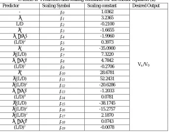
Model

The developed model is given in equation (2). It has 19 different predictor combinations. The modelled wind speed augmentation is strongly correlated to empirical data with R2 = 0.9751 and a root mean square error (RMSE) = 0.





















2 3 4 2 3 4

0 0 1 3 6 10 2 4 7 11 15

2 3

2 3 2

5 8 12 16 9 13 17

4 5

14 18 19

/ x

V V p p p p p p p p p p L D

p p p p L D p p p L D

p p L D p L D

                     _     _   _{  }  _ _{ }  _           (2)

The validity of the model is given in the last column of Table I. Table II shows the values of the scaling constants



p₀p₁₉



of the

predictors of the polynomial regression model equation (2).

TABLE II Predictors and scaling constants for the model equation (2)

Predictor Scaling Symbol Scaling constant Desired Output

- p0 1.0362

Vx /V0

θ p1 3.2365

L/D p2 -0.2100

θ2 p3 -1.6655

θ (L/D) p4 -1.9960

(L/D)2 p5 0.3973

θ3 p6 -35.0900

θ2(L/D) p7 7.3220

θ (L/D)2 p8 4.7842

(L/D)3 p9 -0.2706

θ4 p10 28.6781

θ3(L/D) p11 52.2431

θ2(L/D)2 p12 -20.6286

θ (L/D)3 p13 -1.2033

(L/D)4 _p

14 0.0781

θ4(L/D) p15 -38.1745

θ3

(L/D)2 p16 -15.2757

θ2(L/D)3 p17 2.1870

θ (L/D)4 p18 0.0743

(L/D)5 p19 -0.0078

Mathematical model

(Equations, Algorithms, etc

)

Output

parameters Input

Equation (2) gives the general wind speed augmentation model by empty conical diffusers of 0.5L D3. This model can be

used by DAWT designers to determine the optimum wind speed augmentation by an empty conical diffuser before the turbine rotor is inserted. This enables the designers to optimize the power output of the DAWT system. However, for design purposes, only one L D is needed. Respective model equations can be deduced by substituting the desired L D and the predictor coefficients as given

in Table II in the model equation (2). As an example, a design equation for L D1is given by substituting for L D in equation (2)

and one gets:

2 3 4

0

/ 1.0232 4.8957 12.7851 1.8774 9.4964

x

V V         (3)

Substituting θ values in equation (3), one gets the optimum angle which correspond to L D1, that is, 11o. Therefore, for L D1, to get optimum wind speed augmentation which would give optimum wind power output by the DAWT, the conical diffuser should have an expansion angle of 11o. It should however be emphasized that the θ values should be within the limits of the model as given in the last column of Table I.

B. Ranking of Predictors by Importance of Weight Contribution to Output

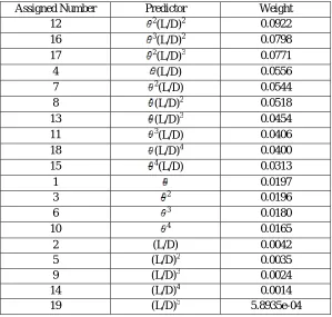
[image:4.612.157.456.393.678.2]

To determine the contribution of the predictors to the model, the Relief algorithm was used. It ranks the predictors according to their weight contribution to the desired output. The Relief algorithm was applied to the 19 terms expressed as predictors and given in Table II. The benefit of ranking predictors using Relief algorithm is to be able to differentiate between primary and secondary contributors. In the Relief Algorithm when the weight of contribution to the output is positive the predictor is said to be a primary contributor. In addition, if the weight of the contribution of the predictor to the output is negative the predictor is said to be a secondary contributor. The weight of contribution by the Relief Algorithm for the predictors ranges between -1 and 1 with large positive weights assigned to important predictors. Table III shows predictors and their assigned numbers according to weight of contribution.

TABLE III Model Predictors ranked by weight of contribution

Assigned Number Predictor Weight

12 2

(L/D)2 0.0922

16 3

(L/D)2 0.0798

17 2(L/D)3 0.0771

4 (L/D) 0.0556

7 2

(L/D) 0.0544

8 (L/D)2 0.0518

13 (L/D)3 0.0454

11 3

(L/D) 0.0406

18 (L/D)4 0.0400

15 4

(L/D) 0.0313

1 0.0197

3 2 _0.0196

6 3 _0.0180

10 4 0.0165

2 (L/D) 0.0042

5 (L/D)2 0.0035

9 (L/D)3 0.0024

14 (L/D)4 0.0014

19 (L/D)5 5.8935e-04

With reference to Table III, it can be seen that predictors that are purelyL D dependent contributed the least with their weight of

contribution decreasing as the power of L D increases. Basing on the Relief weight ranking, Fig. 3 was generated with the Y axis

[image:5.612.148.486.109.279.2]

predictor number as given in equation (2) and the vertical axis gives the corresponding weight of each predictor in the development of the model.

Fig.3. A graph of model predictor ranking

It is observed that all the 19 predictors are primary contributors. The predictors contributing the most are predictors assigned by the

numbers 12, 16 and 17 and this corresponds to 2



L D



2, 3



L D



2and 2



L D



3(with weight contributions of 0.0922, 0.0798

and 0.0771 respectively). The predictors contributing the least by weight are those assigned by the numbers 19, 14 and 9 and this

corresponds to



L D



5,



L D



4 and



L D



3 (with weight contributions of 5.8935e-04, 0.0014 and 0.0024 respectively). It can be

seen that θ as a predictor contributes more to the desired output as compared L D. This means that the diffuser expansion angle is

more important than L D in wind speed augmentation in a conical diffuser.

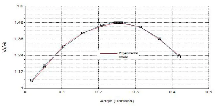
C. Comparison of Experimental Data and the Developed Polynomial Regression Model

The polynomial regression model was compared with the experimental data. Fig. 4 and 5 show graphs of the comparison of the model and the experimental data. Only graphs for L D0.5 andL D3 are shown. For each L D, graphs of the experimental

data and the model, the model equation and the corresponding RMSE are given.

Model equation for L D0.5:

2 3 4

0

/ 1.0013 3.2887 2.8883 12.7874 9.5909 0.039

x

V V          (4)

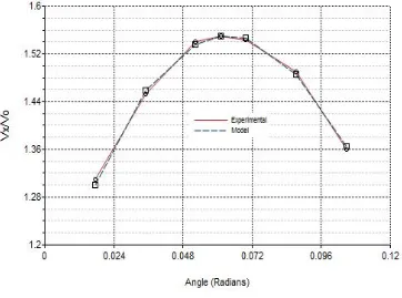
[image:5.612.101.470.533.715.2]

Model equation for L D3:

2 3 4

0 1.1064 13.8355 106.307

/ 9 15.842 85.8454 0.028

x

[image:6.612.104.466.128.397.2]

V V          (5)

Fig. 5 Graphs for the comparison of the model and experimental data for

Equations (4) and (5) give model equations forL D0.5 and L D3 respectively. In Fig. 4



V_x/V_{0 max}



1.48 was achieved at 14.5o (0.252944 rad.) and in Fig. 5,



V_x/V_{0 max}



1.55 was achieved at 3.5o (0.061056 rad). Therefore, 14.5o and 3.5o are the optimum design angles forL D0.5 and L D3 respectively. To achieve optimum wind power output, DAWT ofL D0.5

and L D3 should have diffuser expansion angles of 14.5o and 3.5o respectively. The RMSE was used as the goodness of fit of the model. It gives the average deviation of the model from the experimental data. For L D0.5 a RMSE of 0.039 was obtained and

0.028 for L D3. The deviations are quite minimal. This indicates that the developed model agrees with the experimental data.

The model can reliably be used for conical diffuser design.

IV. CONCLUSION

A polynomial regression model which estimates wind speed augmentation by an empty conical diffuser was developed. The model is useful to DAWT engineers in the design stage of the optimization of the power output of DAWT wind energy systems. Each

L D has its own particular optimum angle which give maximum wind speed augmentation. This is obtained from the

corresponding model equation of that L D. The model and the experimental data were correlated with R2 = 0.9751 and RMSE = 0.034. It was illustrated that the expansion angle (θ) as a predictor contributes more to the desired output as compared to L D. This

means that during the design and construction stages, more attention should be given to the diffuser expansion angle since wind speed augmentation is heavily depended on it.

REFERENCES

[1] G.J.W.V. Bussel, An assessment of the performance of diffuser augmented wind turbines (DAWT), in Proc. 3rd ASME/JSME Joint Fluids Engineering Conference, San Francisco, California, USA, 18-23 July 1999.

[3] K.M. Foreman, B.L. Gilbert, Technical development of the diffuser augmented wind turbine (DAWT) concept, in Wind Energy Innovative Systems Conference Proceedings, Colorado Springs, Colorado, USA, pp. 121-134, 1979

[4] F. M. White, Fluid Mechanics, 7th ed. MacGraw-Hill, Newyork, 2009

[5] F. Owis, M. T. S. Badaway, K. A. Abed, H. E. Fawaz and A.Elfeky, Numerical investigation of loaded and unloaded diffuser equipped with a flange, International Journal of Scientific and Engineering Research, Vol. 6, No. 11, pp.312-341, 2015

[6] S. A. H. Jafari and B. Kosasih, Flow analysis of shrouded small wind turbine with simple frustrum diffuser with computational fluid dynamics simulations, Journal of Wind Engineering and Industrial Aerodynamics, Vol. 125, pp.102-110, 2014

[7] B. Djebedjian, Diffuser optimization using computational fluid dynamics and Micro- genetic algorithms, Mansoura Engineering Journal, Vol. 28, no. 4, 2003.

[8] T. Matsushima, S. Takagi, and S. Muroyama, Characteristics of a highly efficient propeller type small wind turbine with a diffuser, Renewable Energy, Vol. 31, pp. 1343–1354, 2006

[9] R. Chaker, M. Kardous, F. Aloui, and S. B. Nasrallah, Relationship between open angle and aerodynamic performances of a DAWT, in Proc. The Fourth International Renewable Energy Congress, Sousse, Tunisia, 20-22 December 2012.

[10] M. M. Sarwar, N. Nawshin, M. A. Imam, and M. Mashud, A new approach to improve the performance of an existing small wind turbine using diffuser, International Journal of Engineering & Applied Sciences (IJEAS), Vol. 4, no. 1, pp. 31-42, 2012

[11] P. Masukume, G. Makaka, and D. Tinarwo, Optimum geometrical shape parameters for conical diffusers in ducted wind turbines. International Journal of Energy and Power Engineering, Vol. 5 No. 6, pp. 177-181. 2016