UWB Channel Modeling Improvement in Indoor Line of Sight (LOS) Environments

UWB Channel Modeling Improvement in Indoor

Line-of-Sight (LOS) Environments

Vahid Tabataba Vakili, Dariush Abbasi-Moghadam, Mostafa Yahyaabadi

School of Electrical Engineering, Department of Telecommunications, Iran University of Science & Technology (IUST), Narmak, Iran

E-mail: [email protected], [email protected], [email protected] Received August 1, 2010; revised September 19, 2010; accepted October 21, 2010

Abstract

Channel measurement and modeling are important issues when designing ultra wideband (UWB) communi-cation systems. A Precise model of the channel response is inevitable for designing a UWB telecommunica-tion system. In this article signal propagatelecommunica-tion in indoor environment and LOS conditelecommunica-tion is evaluated and the appropriate model of this scenario is presented. Parameters such as the power delay profile, mean excess de-lay, delay spread, “NP10dB” are analyzed and simulated. Based on the analysis results, the proposed model is

presented. This model is based on Two-cluster approach but its average power delay profile is described with power function and cluster time of the arrival is modeled by the modified exponential distribution. Finally UWB channel parameters of the proposed model, Saleh and Valenzuela (S-V) and Two-cluster models are compared. Measurement and simulation results show that considerable improvement for mean excess delay, delay spread and “NP10dB” of proposed model comparing with S-V and Two-cluster models, this means the

channel is better described, which mean the channel is described more precisely.

Keywords:Channel Modeling, S-V Model, Power Delay Profile, Ultra Wideband

1. Introduction

UWB technology has been employed for several decades in military and commercial communications applications like high-speed mobile local area networks, imaging and surveillance systems, ground penetration radars, automo-tive sensors, medical monitors and recently wireless personal area networks. FCC has allocated band width from 3.1 GHz to 10.6 GHz to ultra wideband systems [1]. In recent years, these systems have gained more attention because of their advantages over narrowband systems. This system’s RF signal consists of ultra short pulses with low power spectral density. Low transmission power (–41.3 dBm) and large bandwidth together render the power spectral density of the transmitted signal ex-tremely low, which allows the frequency-overlay of a UWB system with other existing radio systems such as GPS, IEEE802.11x and WLNA [2]. Spread-spectrum communication systems using ultra-short impulses have seen a renewed interest because of its fine resolution in delay to the order of several nanoseconds though at the cost of an ultra wide frequency band.

Channel transmission is a propagation environment

871

model is based on S-V model for ultra wideband channel including several stochastic clusters while in this model only two deterministic clusters are considered. Unfortu-nately, since in Two-cluster model, the second cluster is larger that S-V model clusters, we cannot define the av-erage power delay profile with exponential function. A model has been proposed in this paper in which the av-erage power delay profile is defined by power function.

The paper is organized as follows: in Section 2, meas-urement conditions are explained, in Section 3, Two- cluster and S-V models are introduced, Section 4 pre-sents the proposed model, while in Section 5 new model is simulated and finally concluding remarks are pre-sented in Section 6.

2. Measurement

Propagation measurements have been made to character-ize the UWB signal propagation channel. Using short pulse with sub-nanosecond width, the impulse response of the channel can be observed. Figure 1 is the block diagram of the experimental setup. Transmitter consists of a pulser, a periodic pulse generator, and a transmitting antenna. The periodic pulse generator generates a regular frame clock signal with period of 1 microsecond, which triggers the pulser. The periodic pulse generator is also connected to a DSO (Digitized Sampling Scope) by co-axial cable to provide a trigger signal for a measurement of the receiving antenna output. The pulser generates Gaussian-shaped pulses with sub-nanosecond duration.

Figure 2 shows the output signals of a typical pulser. Since the antenna system differentiates and filters the pulser’s output, a more complex waveform is detected by the DSO. Incoming signal is differentiated at receiving antenna and observed at DSO. The DSO takes samples over many periods of the transmission to construct one received waveform, and averages several such waveform measurements. Figure 2(b) shows a typical signal meas-ured by the DSO in an indoor setting. The LOS path component of the signal is shown in the first two or three nanoseconds of the response, and is followed by a num-ber of multipath components.

Experiments were carried out in a laboratory with size

Figure 1. A block diagram of the measurement apparatus [6].

of 2.7 m (height), 13.5 m (length) and 8.5 m (wide). The transmitter antenna has been located 165 cm far from the floor near the southern wall. LOS receiver, which is named F1, has been located 9.5 meter far from the transmitter, near the western wall. The distance from receiver antenna to floor is 120 cm. In Figure 3, the plan of laboratory has been shown from above. In receiver location, a square matrix of 7 × 7 = 49 sensors with 15 cm spacing has been provided.

CLEAN algorithm was used to extract the CIR from measurements data of the received waveforms [8,9]. The power delay profile [10,11], defined by (1) is averaged over 49 measured channels and is plotted in Figure 4.

2 49

) ( 1



 M

m m

h M

PDP  (1)

Experimental data have been used as criteria for exami-nation of model’s accuracy. Therefore, each model im-pulse response is a random process which cloud be ade-quately presented by three random variables (parameters):

mean excess delay, RMS delay spread NP10dB. CDF and

mean of each parameters are computed by simulation using at least 1000 runs. It is obvious, CDF and mean of a model which is closer to measured CDF and mean will be selected as a more precise channel model as described in the following section.

Figure 3. Plan of laboratory where the LOS propagation measured experiment was performed [7].

Figure 4. Average power delay profile versus excess delay in a semi logarithmic scale for the 49 LOS locations in the laboratory.

3. S-V and Two-Cluster Model

It can be seen from Figure 4, due to multipath compo-nents in UWB systems, each cluster consists of several rays. This definition of ultra wideband systems were in-troduced by “Saleh and Valenzuela” for the first time [3, 11-13]. The following impulse response has been pro-posed for UWB channel [14]:



 

 

 L

l K

k kl l kl

T t X

t h

0 0

, , ( )

)

(    (2)

where L denotes the number of clusters, l is the cluster index, k is ray index, L is total number of clusters, K is the total number of rays in each cluster. X Indicates

shad-owing factor and k,l is ray gain for k

th

ray of lth cluster. These two parameters are modeled by lognormal distri-bution. Also l is lth cluster time arrival, k,l



T  is time

arrival of kth rays of lth cluster. Assuming time of arrival distribution as Poisson, time interval distribution should be considered as exponential.

S-V model has several problems. First, this model is not accurate for LOS and indoor applications. Second, finding the accurate values of parameters like cluster arrival rate and inter cluster exponential decay constant is difficult for modeling cluster behaviors based on ex-perimental data .This would require some specific algo-rithms of distinguishing clusters from one another. In order to compensate for this disadvantage, an UWB channel model with two deterministic clusters and sto-chastic arriving rays within each cluster were proposed [5].This model is based on S-V model, but the only dif-ference is that instead of several clusters with random time of arrival, only two clusters are considered with deterministic time of arrival (Figure 4). Also, instead of determining the gain of first ray of each cluster stochas-tically in S-V model, the gain of first ray in first and second clusters are computed deterministically. The other model components, i.e., gain and time of arrival of next rays in each two cluster are modeled statistically. The channel has the following response:





 



  



 1

0

1 , 1

, 1

0

0 , 0

, ( ) ( )

) (

N

k k m k

M

k k k

T t t

t

h       (3)

where k,l is multipath gain coefficient, Tm is the time interval between two clusters, k,0



 is the delay of the

kth multipath component relative to the first cluster arri-val time, k,l is the time delay of the kth multipath

component relative to the second cluster arrival time (Tm),

M is the number of paths in the first cluster, and N is the number of paths in the second cluster. The parameters of this model can be divided into deterministic and stochas-tic parts. In order to calculate the determinisstochas-tic parame-ters, it is enough to have length, width and height of the room, electromagnetic properties of reflecting surface, polarization and bandwidth of transmitted and received signal. The statistical parameters are modeled like S-V model.

4. Proposed Model

873

4.1. Deterministic Part of Model

Deterministic part of the model includes the path gain of the first ray of two clusters and their time delay. In this model, LOS ray is considered as the first ray of the first cluster. The arrival time of this ray is assumed to be zero and its gain is determined based on path loss characteris-tic of free space:

m f c d       , 4 0 ,

0 (4)

where c is light speed, fmis the geometrical mean of the upper and lower signal frequency limits, d is the distance between the transmitter and receivers’ antenna. The first ray of the second cluster is a ray which is reflected once from six reflecting surfaces (four walls, ceiling and floor of laboratory). The arrival time of this ray is calculated as follows:

0

min{ }

, 1, 2, 3, 4, 5, 6

i m L L T i C 

  (5)

where L₀is the length of direct path and Liis the length

of reflected rays. For computing the gain of this ray ex-cept path loss of free space, we should consider the loss resulting from reflection [15]. Therefore:

0 0,1 0 2 min{ } 2

1 exp[(1 ) ] , 1...6

1 i m L L L k

K K aT

k        _   _      

 i

(6)

With K =(1-k)/(1+k), and

    sin cos2    r r

k for

ver-tical polarization and

   2 cos sin   r

k for horizontal

polarization and a120  c/ _r. Here, r and are

relative dielectric constant and the conductivity of re-flecting surface [16] respectively. By the abovemen-tioned definitions, the deterministic parameters are cal-culated and presented in Table 1.

4.2. Statistical Part of Model

The gain and arrival time of the next rays in both clusters are modeled statistically. The gain of these rays is mod-eled as follows, but with slight difference with S-V model: 1 , 1 / 0 , 1 / 0 , 1 / 0

, Pk k k

k 

 (7)

where Pk,0/1 will be 1 with equal probability. k,0/1

is lognormal fading of rays with standard deviation of δ:

1 ), , ( ) ( log

20 k,0/1 Normal k,0/12 k

1 / 0 , k  (8)

Determination of depends on the fun

ty of average power delay profile. In Two-cluste

od wer

ctionali r m

el, the average po delay profile is defined by

exponential function:





1 / 0 , 2 1 / 0 ,   E k k  

 2 0/1

1 / 0 ,

0 e k



(9)

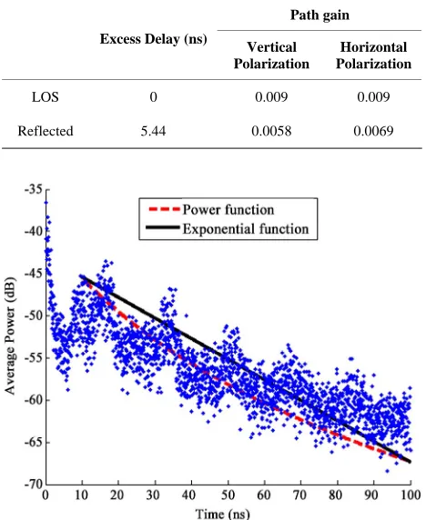
As Figure 5 shows, the average power does not follow the exponential function accurately co

delay profile (the ntinuous line shows the exponential function). The reason why is the fact that the second large cluster con-sists of several small clusters are not considered in mod-eling of the average PDP as exponential function of time. In order to achieve more accuracy, we define the av-erage power delay profile as a power function of time:





 k m

k

T

E 2 ,0/1

1 / 0 , 0 2 1 / 0

, ( ) (1



 Tm

0)

where k,l is ray gain for multi-path, k,l is arrival

time rays of lth cluster and T ime

own in Figure 5. The dashed line shows

po

of kth m

arrival t .

The adjustment of power delay profile with power function is sh

is the second cluster

wer function. As Figure 5 shows, the average power

Table 1. Values of deterministic parameters of model.

Path gain Ho Pola al tion rizontal rization Vertic Polariza Excess Delay (ns)

0.009 0.009 0 LOS 0.0069 0.0058 5. Reflected 44

delay profile based on power function, compared with exponential, is more fitted to measured PDP data. The mean and variance of error between averaged PDP based on power function and measured PDP and also error be-tween averaged PDP based on exponential function and

measured PDP are presented in Table 2. As this table

shows the difference between variances of these two function models is 2.0166 dB respectively. Hence we should compute k,l based on new definition of

aver-age power delay profile.

Since k,0/1is modeled with lognormal distribution

(Equation 8), we can have:

) , ( . 10 ) 10 ln( 2 1 / 0 , 2  

k e Nor 1 / 0 , k mal (11) Hence: (12)

From (12) and (13) we have:

 

2 2

), ,

( B mb b

b

b z e Ez e

m     

Normal B ) , ( ) ,

(m2 Normal km k22 Normal

k  (13)

2 2 2 1 / 0 , ) ( 2 2 1 / 0 , ] ,

[ e 

E m Var

k ) 20 ( )) 10 (ln( , 20 ). 10

ln(  



 Var

m k (14)

By equalizing (10) and (14) we conclude that:

20 ) 10 ln( ) 10 ln( ) ln( 10 ln

20 0,0/1 ,0/1 _2

,

 

  k Tm

  m 

l k

T

(15)

Therefore, in the proposed model is the

no

k,0/1

 ion

log-rmal fading term with standard deviat  and k,l

which was defined in (Equation 15). Arrival time of ray in Two-cluster model described with exponential func-tion, but in proposed model, arrival time of rays de-scribed with modified exponential function (Equation 16). Comparison of arrival time of ray of these two mod-els with measured data shows that the proposed model is improved. So in the proposed model, the time interval between times of rays’ arrival is modeled with modified exponential distribution:

,0/1 1,0/1

( _k | _k ) (1 ) exp( ( ))

P    b    



1 1 ,0/1 1,0/1

2 exp( 2( ,0/1 1,0/1))

k k k k b           (16)

where b is close to 1. The values of ,,,b, n in Table 3

w

esult of Two-cluster model, -V model and the proposed model have been compared.

ariances of error.

wer function

hich

were used in simulation have been show .

5. Simulation Results

I S

n this section simulation r

This comparison has been done regarding mean and

cu-mulative distribution function of three key parameters, i.e., mean excess delay, RMS delay spread and “NP10dB”.

First, several channels have been simulated for both pre-vious models and proposed model by MATLAB 7 Then the parameters of each simulated channel are computed and recorded and the mean and cumulative distribution function for each parameter was obtained from these recorded values. In order to compare and evaluate these models, the obtained values of mean and cumulative dis-tribution function in measured data have been considered as reference. In Table 4 the result of mean value of pa-rameters is compared. The average value of mean excess delay in the proposed model, Two-cluster model and S-V model are 14.68 ns, 15.28 ns and 16.04 ns, respectively. Also, the mean value for RMS delay spread in the pro-posed model, Two-cluster model and S-V model are 17.54 ns 17.62 ns and 18.76 ns, respectively. The mean

value of “NP10dB” in the proposed model, Two-cluster

model and S-V model are 7.85, 8.91 and 8.93, respec-tively and “NP10dB” in measured data is 7.51. Compare

these values with obtained values from measurements show that the average relative error proposed model pa-rameters, mean excess delay and delay spread and

“NP10dB” in comparison with the Two-cluster model

were 4.2 percent, 0.45 percent, 14.11 percent, compared S-V model, respectively, 9.5 percent, 6.88 percent and 14.38 percent decrease.

Table 2. V

Po Exponential function

22.2731 24.2897

error variance

Tab aramete proposed mod

imu-tion.

le 3. Value of p rs used in el s

la

0.15

(1 / ns) 1 

1.54

2(1 / ns) 

0.

b 095

17.6 (ns)  3.3941 (dB) 

Table 4. Average value of key parameter.

875

Figure 6. CDF of mean excess delay.

Figure 7. CDF of RMS delay spread.

Figure 8. CDF of number of significant multipaths.

In Figures 6-8 the CDF of mean excess delay, RMS

delay spread and “NP10dB” have been drawn for three

models. As it can be seen, CDF of mean excess delay and RMS delay spread in the proposed model is closer to the measured values than Two-cluster model and S-V model. Also CDF of “NP10dB” is better for the proposed

model comparing to the previous models. The ray arrival time in the proposed model, which is described with ex-ponential distribution using 1, 2, is more precise

compared to S-V and Two-cl odels. Furthermore,

the ray arrival time and the ray gain of the proposed model are closer to the experimental results.

6. Conclusion

In this paper, a model has been presented for indoor LOS

UW OS

U

t o

he modified n. Results show that the cumulative ons of three parameters of proposed odel has been recovered comparing with S-V model

uster m

B channel. The proposed model for indoor L WB channel doesn't need the description of clusters and knowing the mean parameters of arrival rate of clus-ter and their variance comparing to S-V model. Also, instead of approximating the gain of first ray with a mean value, it is determined accurately and substituted in the model. Moreover instead of simulating the time arri-val of several clusters with statistical distribution, we should compute deterministically and use the time arrival of two clusters. As in Two-clus er m del, several clusters of S-V model are considered as the second cluster. In proposed model, the average power delay profile was approximated with power function. Furthermore in the

oposed model, times were modeled by t pr

exponential functio distribution functi m

and Two-cluster model. The mean value for mean excess

delay and RMS delay spread and “NP10dB” in the

pro-posed model have been recovered 0.6 ns, 0.08 ns and 1.06 comparing with Two-cluster model and 1.36 ns, 1.22 ns and 1.08 comparing with S-V model. Therefore the proposed model fits better for data and has less vari-ance, hence it can model the channel better than S-V and Two-cluster model in LOS environment.

7. References

[1] M. Z. Win and R. A. Scholtz, “Characterization of Ul-tra-Wide Band Width Wireless Indoor Communication Channel: A Communication Theoretical View,” IEEE JSAC, Vol. 20, No. 9, December 2002, pp. 1613-1627. [2] Multiband OFDM Physical Layer Proposal for IEEE

802.15 Task Group 3a. http://www.ieee802.org/15/

Systems Engi-lectronics, Vol. 18, No. 4, December 2007,

tromagnetic Compatibility, Vol. 46, No. 4,

” IEEE 19th International

of the Power Delay Profile,” Elsevier

Interna-3a, 2002. [4] S. Venkatesh and J. Ibrahim, “A New 2-Cluster Model for

Indoor UWB Channel Measurement,” IEEE in Antenna and Propagation Society Symposium, Vol. 1, June 2004, pp. 946-949.

[5] Y. Wang, N. T. Zhang, Q. Y. Zhang and Z. Z. Zhang, “Characterizing Ultra-Wide Band Indoor Line-of-Sight Wireless Channel,” Elsevier Journal of

neering and E pp. 673-678.

[6] http://ultra.usc.edu/uwb_database/

[7] D. Cassioli, M. Z. Win and A. F. Molisch, “The Ul-tra-Wide Bandwidth indoor Channel: From Statistical Model to Simulations,” IEEE Journal on Selected Areas in Communications, Vol. 20, No. 6, August 2002, pp. 1247-1257.

[8] Y. Wang and N. T. Zhang, “A New Multi-Template CLEAN Algorithm for UWB Channel Impulse Response Characterization,” IEEE Conference on Communication Technology, Guilin, November 2006, pp. 1-4.

[9] C. Buccella, M. Feliziani and G. Manzi, “Detection and Localization of Defects in Shielded Cables by Time-Domain Measurement with UWB Pulse Injection and Clean Algorithm Post Processing,” IEEE Transac-tions on Elec

of Tr

November 2004, pp. 597-605.

[10]J. H. Kim and Y. K. Yoon, “The Multipath Delay Spread Model for the LOS Case,” Antennas and Propagation Society International Symposium, San Diego, July 2008, pp. 1-4.

[11]R. G. Vaughan and N. L. Scott, “Super-Resolution of Pulsed Multipath Channels for Delay Spread Characteri-zation,” IEEE Transactions on Communications, March 1995, Vol. 47, No. 3, pp. 343-347.

[12]Y. F. Chen, “Statistical Properties of IEEE UWB Channel Models and Their Application,

Symposium on Indoor and Mobile Radio Communica-tions, Cannes, September 2008, pp. 1-5.

[13]J. Wout, D. Jeffrey, V. Leen and M. Luc. “Statistical Analysis

tional Journal of Communications, In Press, Available online, 7 July 2009.

[14] J. Foerster, “Channel Modeling Sub-Committee Report Final,” IEEE P802.15-02/368r5-SG

[15]V. Marshall and G. Skitek, “Electromagnetic Concept and Applications,” Prentice-Hall International, Inc., 1990.