Numerical Methods in Engineering with Python
Second Edition
Numerical Methods in Engineering with Python, Second Edition, is a text for engineering students and a reference for practicing engineers, especially those who wish to explore Python. This new edition fea-tures 18 additional exercises and the addition of rational function in-terpolation. Brent’s method of root finding was replaced by Ridder’s method, and the Fletcher–Reeves method of optimization was dropped in favor of the downhill simplex method. Each numerical method is explained in detail, and its shortcomings are pointed out. The ex-amples that follow individual topics fall into two categories: hand computations that illustrate the inner workings of the method and small programs that show how the computer code is utilized in solv-ing a problem. This second edition also includes more robust com-puter code with each method, which is available on the book Web site (www.cambridge.org/kiusalaaspython). This code is made simple and easy to understand by avoiding complex bookkeeping schemes, while maintaining the essential features of the method.
Jaan Kiusalaas is a Professor Emeritus in the Department of Engineer-ing Science and Mechanics at Pennsylvania State University. He has taught computer methods, including finite element and boundary el-ement methods, for more than 30 years. He is also the co-author of four other books –Engineering Mechanics: Statics, Engineering Mechanics: Dynamics, Mechanics of Materials, and an alternate version of this work with MATLABR
code.
NUMERICAL
METHODS IN
ENGINEERING
WITH PYTHON
Second Edition
Jaan Kiusalaas
Pennsylvania State University
iv
CAMBRIDGE UNIVERSITY PRESS
Cambridge, New York, Melbourne, Madrid, Cape Town, Singapore, São Paulo, Delhi, Dubai, Tokyo
Cambridge University Press
The Edinburgh Building, Cambridge CB2 8RU, UK
First published in print format
ISBN-13 978-0-521-19132-6 ISBN-13 978-0-511-68592-7
© Jaan Kiusalaas 2010
2010
Information on this title: www.cambridge.org/9780521191326
This publication is in copyright. Subject to statutory exception and to the provision of relevant collective licensing agreements, no reproduction of any part may take place without the written permission of Cambridge University Press.
Cambridge University Press has no responsibility for the persistence or accuracy of urls for external or third-party internet websites referred to in this publication, and does not guarantee that any content on such websites is, or will remain, accurate or appropriate.
Published in the United States of America by Cambridge University Press, New York www.cambridge.org
Contents
Preface to the First Edition . . . .viii
Preface to the Second Edition . . . .x
1 Introduction to Python . . . .1
1.1 General Information . . . .1
1.2 Core Python . . . .3
1.3 Functions and Modules . . . .15
1.4 Mathematics Modules . . . .17
1.5 numpyModule . . . .18
1.6 Scoping of Variables . . . .24
1.7 Writing and Running Programs . . . .25
2 Systems of Linear Algebraic Equations . . . .27
2.1 Introduction . . . .27
2.2 Gauss Elimination Method . . . 33 2.3 LU Decomposition Methods . . . .40
Problem Set 2.1. . . .51
2.4 Symmetric and Banded Coefficient Matrices . . . .54
2.5 Pivoting . . . .64
Problem Set 2.2. . . .73
∗2.6 Matrix Inversion . . . .79
∗2.7 Iterative Methods . . . .82
Problem Set 2.3. . . .93
∗2.8 Other Methods . . . .97
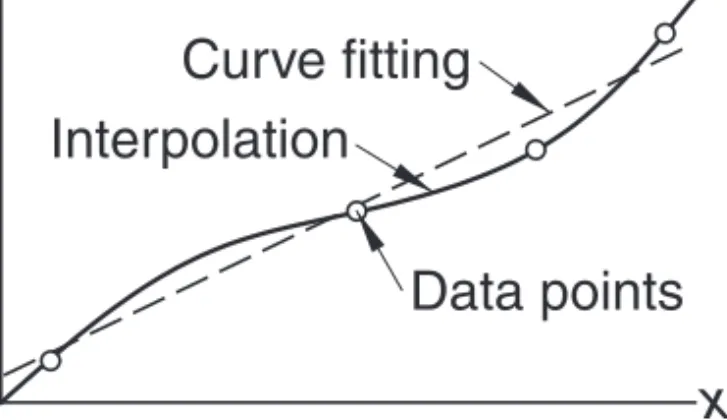
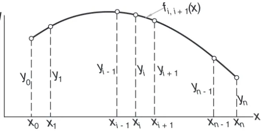
3 Interpolation and Curve Fitting . . . .99
3.1 Introduction . . . .99
3.2 Polynomial Interpolation. . . .99
3.3 Interpolation with Cubic Spline . . . .114
Problem Set 3.1. . . .121
3.4 Least-Squares Fit . . . .124 Problem Set 3.2 . . . 135 4 Roots of Equations . . . .139
4.1 Introduction . . . .139
4.2 Incremental Search Method . . . .140
4.3 Method of Bisection. . . .142
4.4 Methods Based on Linear Interpolation . . . .145
4.5 Newton–Raphson Method . . . .150
4.6 Systems of Equations . . . 155 Problem Set 4.1. . . .160
∗4.7 Zeroes of Polynomials . . . .166
Problem Set 4.2. . . .174
5 Numerical Differentiation . . . .177
5.1 Introduction . . . .177
5.2 Finite Difference Approximations. . . .177
5.3 Richardson Extrapolation . . . .182
5.4 Derivatives by Interpolation . . . .185
Problem Set 5.1. . . .189
6 Numerical Integration. . . .193
6.1 Introduction . . . .193
6.2 Newton–Cotes Formulas . . . .194
6.3 Romberg Integration . . . .202
Problem Set 6.1. . . .207
6.4 Gaussian Integration . . . .211
Problem Set 6.2. . . .225
∗6.5 Multiple Integrals. . . .227
Problem Set 6.3. . . .239
7 Initial Value Problems . . . .243
7.1 Introduction . . . .243
7.2 Taylor Series Method . . . .244
7.3 Runge–Kutta Methods . . . .249
Problem Set 7.1. . . .260
7.4 Stability and Stiffness . . . .266
7.5 Adaptive Runge–Kutta Method . . . .269
7.6 Bulirsch–Stoer Method . . . .277
Problem Set 7.2. . . .284
7.7 Other Methods . . . .289
8 Two-Point Boundary Value Problems . . . .290
8.1 Introduction . . . .290
8.2 Shooting Method . . . .291
Problem Set 8.1. . . .301
8.3 Finite Difference Method . . . .305
Problem Set 8.2. . . .314
9 Symmetric Matrix Eigenvalue Problems . . . .319
9.1 Introduction . . . .319
9.2 Jacobi Method . . . .321
9.3 Power and Inverse Power Methods . . . .337
Problem Set 9.1. . . .345
9.4 Householder Reduction to Tridiagonal Form . . . .351
vii Contents
Problem Set 9.2. . . .367
9.6 Other Methods . . . .373
10 Introduction to Optimization . . . .374
10.1 Introduction . . . .374
10.2 Minimization along a Line . . . .376
10.3 Powell’s Method . . . .382
10.4 Downhill Simplex Method . . . .392
Problem Set 10.1. . . .399
10.5 Other Methods . . . .406
A1 Taylor Series . . . .407
A2 Matrix Algebra. . . .410
List of Program Modules (by Chapter) . . . .416
Preface to the First Edition
This book is targeted primarily toward engineers and engineering students of ad-vanced standing (juniors, seniors, and graduate students). Familiarity with a com-puter language is required; knowledge of engineering mechanics (statics, dynamics, and mechanics of materials) is useful, but not essential.
The text attempts to place emphasis on numerical methods, not programming. Most engineers are not programmers, but problem solvers. They want to know what methods can be applied to a given problem, what are their strengths and pitfalls, and how to implement them. Engineers are not expected to write computer code for basic tasks from scratch; they are more likely to utilize functions and subroutines that have been already written and tested. Thus, programming by engineers is largely confined to assembling existing bits of code into a coherent package that solves the problem at hand.
The “bit” of code is usually a function that implements a specific task. For the user the details of the code are unimportant. What matters is the interface (what goes in and what comes out) and an understanding of the method on which the algorithm is based. Since no numerical algorithm is infallible, the importance of understanding the underlying method cannot be overemphasized; it is, in fact, the rationale behind learning numerical methods.
This book attempts to conform to the views outlined above. Each numerical method is explained in detail and its shortcomings are pointed out. The examples that follow individual topics fall into two categories: hand computations that illus-trate the inner workings of the method, and small programs that show how the com-puter code is utilized in solving a problem. Problems that require programming are marked with.
The material consists of the usual topics covered in an engineering course on numerical methods: solution of equations, interpolation and data fitting, numerical differentiation and integration, and solution of ordinary differential equations and eigenvalue problems. The choice of methods within each topic is tilted toward rel-evance to engineering problems. For example, there is an extensive discussion of symmetric, sparsely populated coefficient matrices in the solution of simultaneous equations. In the same vein, the solution of eigenvalue problems concentrates on methods that efficiently extract specific eigenvalues from banded matrices.
ix Preface to the First Edition
An important criterion used in the selection of methods was clarity. Algorithms requiring overly complex bookkeeping were rejected regardless of their efficiency and robustness. This decision, which was taken with great reluctance, is in keeping with the intent to avoid emphasis on programming.
The selection of algorithms was also influenced by current practice. This disqual-ified several well-known historical methods that have been overtaken by more recent developments. For example, the secant method for finding roots of equations was omitted as having no advantages over Ridder’s method. For the same reason, the mul-tistep methods used to solve differential equations (e.g., Milne and Adams methods) were left out in favor of the adaptive Runge–Kutta and Bulirsch–Stoer methods.
Notably absent is a chapter on partial differential equations. It was felt that this topic is best treated by finite element or boundary element methods, which are outside the scope of this book. The finite difference model, which is commonly introduced in numerical methods texts, is just too impractical in handling multi-dimensional boundary value problems.
As usual, the book contains more material than can be covered in a three-credit course. The topics that can be skipped without loss of continuity are tagged with an asterisk (*).
Preface to the Second Edition
The major change in the second edition is the replacement of NumArray (a Python extension that implements array objects) with NumPy. As a consequence, most rou-tines listed in the text required some code changes. The reason for the changeover is the imminent discontinuance of support for NumArray and its predecessor Numeric.
We also took the opportunity to make a few changes in the material covered:
• Rational function interpolation was added to Chapter 3.
• Brent’s method of root finding in Chapter 4 was replaced byRidder’s method. The full-blown algorithm of Brent is a complicated procedure involving elaborate bookkeeping (a simplified version was presented in the first edition). Ridder’s method is as robust and almost as efficient as Brent’s method, but much easier to understand.
• The Fletcher–Reeves method of optimization was dropped in favor of the down-hill simplex methodin Chapter 10. Fletcher–Reeves is a first-order method that requires knowledge of the gradients of the merit function. Because there are few practical problems where the gradients are available, the method is of limited utility. The downhill simplex algorithm is a very robust (but slow) zero-order method that often works where faster methods fail.
1
Introduction to Python
1.1
General Information
Quick Overview
This chapter is not a comprehensive manual of Python. Its sole aim is to provide suf-ficient information to give you a good start if you are unfamiliar with Python. If you know another computer language, and we assume that you do, it is not difficult to pick up the rest as you go.
Python is an object-oriented language that was developed in the late 1980s as a scripting language (the name is derived from the British television showMonty Python’s Flying Circus). Although Python is not as well known in engineering circles as some other languages, it has a considerable following in the programming com-munity – in fact, Python is used by more programmers than Fortran. Python may be viewed as an emerging language, because it is still being developed and refined. In the current state, it is an excellent language for developing engineering applications – Python’s facilities for numerical computation are as good as those of Fortran or MATLAB.R
Python programs are not compiled into machine code, but are run by an in-terpreter.1The great advantage of an interpreted language is that programs can be
tested and debugged quickly, allowing the user to concentrate more on the princi-ples behind the program and less on programming itself. Because there is no need to compile, link, and execute after each correction, Python programs can be devel-oped in a much shorter time than equivalent Fortran or C programs. On the negative side, interpreted programs do not produce stand-alone applications. Thus, a Python program can be run only on computers that have the Python interpreter installed.
Python has other advantages over mainstream languages that are important in a learning environment:
• Python is open-source software, which means that it isfree; it is included in most Linux distributions.
1 The Python interpreter also compilesbyte code, which helps to speed up execution somewhat.
• Python is available for all major operating systems (Linux, Unix, Windows, Mac OS, etc.). A program written on one system runs without modification on all systems.
• Python is easier to learn and produces more readable code than do most lan-guages.
• Python and its extensions are easy to install.
Development of Python was clearly influenced by Java and C++, but there is also a remarkable similarity to MATLAB (another interpreted language, very popular in scientific computing). Python implements the usual concepts of object-oriented lan-guages such as classes, methods, and inheritance. We will not use object-oriented programming in this text. The only object that we need is the N-dimensionalarray available in the NumPy module (the NumPy module is discussed later in this chapter).
To get an idea of the similarities between MATLAB and Python, let us look at the codes written in the two languages for solution of simultaneous equationsAx=bby Gauss elimination. Here is the function written in MATLAB:
function x] = gaussElimin(a,b) n = length(b);
for k = 1:n-1 for i= k+1:n
if a(i,k) ˜= 0
lam = a(i,k)/a(k,k);
a(i,k+1:n) = a(i,k+1:n) - lam*a(k,k+1:n); b(i)= b(i) - lam*b(k);
end end end
for k = n:-1:1
b(k) = (b(k) - a(k,k+1:n)*b(k+1:n))/a(k,k); end
x = b;
The equivalent Python function is:
from numpy import dot def gaussElimin(a,b):
n = len(b)
for k in range(0,n-1): for i in range(k+1,n):
if a[i,k] != 0.0:
lam = a [i,k]/a[k,k]
3 1.2 Core Python
for k in range(n-1,-1,-1):
b[k] = (b[k] - dot(a[k,k+1:n],b[k+1:n]))/a[k,k] return b
The commandfrom numpy import dot instructs the interpreter to load the functiondot (which computes the dot product of two vectors) from the module
numpy. The colon (:) operator, known as theslicing operatorin Python, works the same way it does in MATLAB and Fortran90 – it defines a slice of an array.
The statementfor k = 1:n-1in MATLAB creates a loop that is executed with k=1, 2,. . .,n−1. The same loop appears in Python as for k in range(n-1). Here the functionrange(n-1)creates the list [0, 1,. . .,n−2];kthen loops over the elements of the list. The differences in the ranges ofkreflect the native offsets used for arrays. In Python, all sequences havezero offset, meaning that the index of the first element of the sequence is always 0. In contrast, the native offset in MATLAB is 1.
Also note that Python has noendstatements to terminate blocks of code (loops, subroutines, etc.). The body of a block is defined by itsindentation; hence indenta-tion is an integral part of Python syntax.
Like MATLAB, Python iscase sensitive. Thus, the namesnandNwould represent different objects.
Obtaining Python
The Python interpreter can be downloaded from the Python Language Website
www.python.org. It normally comes with a nice code editor calledIdlethat allows you to run programs directly from the editor. For scientific programming, we also need theNumPymodule, which contains various tools for array operations. It is ob-tainable from the NumPy home pagehttp://numpy.scipy.org/. Both sites also provide documentation for downloading. If you use Linux, it is very likely that Python is already installed on your machine (but you must still download NumPy).
You should acquire other printed material to supplement the on-line doc-umentation. A commendable teaching guide is Python by Chris Fehly (Peachpit Press, CA, 2002). As a reference,Python Essential Reference by David M. Beazley (New Riders Publishing, 2001) is recommended. By the time you read this, newer editions may be available. A useful guide to NumPy is found at http://www. scipy.org/Numpy Example List.
1.2
Core Python
Variables
it not so in Python, where variables aretyped dynamically. The following interactive session with the Python interpreter illustrates this (>>>is the Python prompt):
>>> b = 2 # b is integer type >>> print b
2
>>> b = b*2.0 # Now b is float type >>> print b
4.0
The assignmentb = 2creates an association between the nameband the in-tegervalue 2. The next statement evaluates the expressionb*2.0and associates the result withb; the original association with the integer 2 is destroyed. Nowbrefers to thefloatingpoint value 4.0.
The pound sign (#) denotes the beginning of acomment– all characters between # and the end of the line are ignored by the interpreter.
Strings
A string is a sequence of characters enclosed in single or double quotes. Strings are concatenatedwith the plus (+) operator, whereasslicing(:) is used to extract a por-tion of the string. Here is an example:
>>> string1 = ’Press return to exit’ >>> string2 = ’the program’
>>> print string1 + ’ ’ + string2 # Concatenation Press return to exit the program
>>> print string1[0:12] # Slicing Press return
A string is animmutableobject – its individual characters cannot be modified with an assignment statement, and it has a fixed length. An attempt to violate im-mutability will result inTypeError, as shown here:
>>> s = ’Press return to exit’ >>> s[0] = ’p’
Traceback (most recent call last): File ’’<pyshell#1>’’, line 1, in ?
s[0] = ’p’
TypeError: object doesn’t support item assignment
Tuples
5 1.2 Core Python
example, x = (2,). Tuples support the same operations as strings; they are also im-mutable. Here is an example where the tuplereccontains another tuple(6,23,68):
>>> rec = (’Smith’,’John’,(6,23,68)) # This is a tuple >>> lastName,firstName,birthdate = rec # Unpacking the tuple >>> print firstName
John
>>> birthYear = birthdate[2] >>> print birthYear
68
>>> name = rec[1] + ’ ’ + rec[0] >>> print name
John Smith
>>> print rec[0:2] (’Smith’, ’John’)
Lists
A list is similar to a tuple, but it ismutable, so that its elements and length can be changed. A list is identified by enclosing it in brackets. Here is a sampling of opera-tions that can be performed on lists:
>>> a = [1.0, 2.0, 3.0] # Create a list >>> a.append(4.0) # Append 4.0 to list >>> print a
[1.0, 2.0, 3.0, 4.0]
>>> a.insert(0,0.0) # Insert 0.0 in position 0 >>> print a
[0.0, 1.0, 2.0, 3.0, 4.0]
>>> print len(a) # Determine length of list 5
>>> a[2:4] = [1.0, 1.0, 1.0] # Modify selected elements >>> print a
[0.0, 1.0, 1.0, 1.0, 1.0, 4.0]
Ifais a mutable object, such as a list, the assignment statementb = adoes not result in a new objectb, but simply creates a new reference toa. Thus any changes made tobwill be reflected ina. To create an independent copy of a lista, use the statementc = a[:], as shown here:
>>> a = [1.0, 2.0, 3.0]
>>> b = a # ’b’ is an alias of ’a’ >>> b[0] = 5.0 # Change ’b’
>>> print a
>>> c[0] = 1.0 # Change ’c’ >>> print a
[5.0, 2.0, 3.0] # ’a’ is not affected by the change
Matrices can be represented as nested lists with each row being an element of the list. Here is a 3×3 matrixain the form of a list:
>>> a = [[1, 2, 3], \ [4, 5, 6], \ [7, 8, 9]]
>>> print a[1] # Print second row (element 1) [4, 5, 6]
>>> print a[1][2] # Print third element of second row 6
The backslash (\) is Python’s continuation character. Recall that Python se-quences have zero offset, so thata[0]represents the first row,a[1]the second row, and so forth. With very few exceptions, we do not use lists for numerical arrays. It is much more convenient to employarray objectsprovided by the NumPy module. Array objects are discussed later.
Arithmetic Operators
Python supports the usual arithmetic operators:
+ Addition
− Subtraction
∗ Multiplication
/ Division
∗∗ Exponentiation % Modular division
Some of these operators are also defined for strings and sequences as illustrated here:
>>> s = ’Hello ’ >>> t = ’to you’ >>> a = [1, 2, 3]
>>> print 3*s # Repetition Hello Hello Hello
>>> print 3*a # Repetition [1, 2, 3, 1, 2, 3, 1, 2, 3]
>>> print a + [4, 5] # Append elements [1, 2, 3, 4, 5]
>>> print s + t # Concatenation Hello to you
7 1.2 Core Python
Traceback (most recent call last): File ’’<pyshell#9>’’, line 1, in ?
print n + s
TypeError: unsupported operand types for +: ’int’ and ’str’
Python 2.0 and later versions also haveaugmented assignment operators, such as a+ =b, that are familiar to the users of C. The augmented operators and the equiva-lent arithmetic expressions are shown in the following table.
a += b a = a + b a -= b a = a - b a *= b a = a*b a /= b a = a/b a **= b a = a**b a %= b a = a%b
Comparison Operators
The comparison (relational) operators return 1 for true and 0 for false. These opera-tors are:
< Less than
> Greater than
<= Less than or equal to
>= Greater than or equal to
== Equal to
!= Not equal to
Numbers of different type (integer, floating point, etc.) are converted to a common type before the comparison is made. Otherwise, objects of different type are consid-ered to be unequal. Here are a few examples:
>>> a = 2 # Integer
>>> b = 1.99 # Floating point >>> c = ’2’ # String
>>> print a > b 1
>>> print a == c 0
>>> print (a > b) and (a != c) 1
Conditionals
Theifconstruct
if condition:
block
executes a block of statements (which must be indented) if the condition returns true. If the condition returns false, the block is skipped. Theifconditional can be followed by any number ofelif(short for “else if”) constructs
elif condition:
block
which work in the same manner. Theelseclause
else:
block
can be used to define the block of statements that are to be executed if none of the if-elif clauses is true. The function sign of a illustrates the use of the conditionals:
def sign_of_a(a): if a < 0.0:
sign = ’negative’ elif a > 0.0:
sign = ’positive’ else:
sign = ’zero’ return sign
a = 1.5
print ’a is ’ + sign_of_a(a)
Running the program results in the output
a is positive
Loops
Thewhileconstruct
whilecondition:
block
9 1.2 Core Python
again. This process is continued until the condition becomes false. Theelseclause
else:
block
can be used to define the block of statements that are to be executed if the condition is false. Here is an example that creates the list [1, 1/2, 1/3,. . .]:
nMax = 5 n = 1
a = [] # Create empty list while n < nMax:
a.append(1.0/n) # Append element to list n = n + 1
print a
The output of the program is
[1.0, 0.5, 0.33333333333333331, 0.25]
We met theforstatement before in Section 1.1. This statement requires a tar-get and a sequence (usually a list) over which the tartar-get loops. The form of the construct is
for tar get in sequence: block
You may add anelseclause that is executed after theforloop has finished. The previous program could be written with theforconstruct as
nMax = 5 a = []
for n in range(1,nMax): a.append(1.0/n) print a
Herenis the target and the list [1, 2,. . .,nMax−1], created by calling therange
function, is the sequence.
Any loop can be terminated by thebreakstatement. If there is anelsecause associated with the loop, it is not executed. The following program, which searches for a name in a list, illustrates the use ofbreakandelsein conjunction with afor
loop:
list = [’Jack’, ’Jill’, ’Tim’, ’Dave’]
name = eval(raw_input(’Type a name: ’)) # Python input prompt for i in range(len(list)):
if list[i] == name:
else:
print name,’is not on the list’
Here are the results of two searches:
Type a name: ’Tim’
Tim is number 3 on the list
Type a name: ’June’ June is not on the list
The
continue
statement allows us to skip a portion of the statements in an iterative loop. If the interpreter encounters thecontinuestatement, it immediately returns to the begin-ning of the loop without executing the statements belowcontinue. The following example compiles a list of all numbers between 1 and 99 that are divisible by 7.
x = [] # Create an empty list for i in range(1,100):
if i%7!= 0: continue # If not divisible by 7, skip rest of loop x.append(i) # Append i to the list
print x
The printout from the program is
[7, 14, 21, 28, 35, 42, 49, 56, 63, 70, 77, 84, 91, 98]
Type Conversion
If an arithmetic operation involves numbers of mixed types, the numbers are au-tomatically converted to a common type before the operation is carried out. Type conversions can also be achieved by the following functions:
int(a) Convertsato integer
long(a) Convertsato long integer
float(a) Convertsato floating point
complex(a) Converts to complexa+0j
complex(a,b) Converts to complexa+bj
The foregoing functions also work for converting strings to numbers as long as the literal in the string represents a valid number. Conversion from a float to an inte-ger is carried out by truncation, not by rounding off. Here are a few examples:
11 1.2 Core Python
>>> d = ’4.0’ >>> print a + b 1.4
>>> print int(b) -3
>>> print complex(a,b) (5-3.6j)
>>> print float(d) 4.0
>>> print int(d) # This fails: d is not Int type Traceback (most recent call last):
File ’’<pyshell#7>’’, line 1, in ? print int(d)
ValueError: invalid literal for int(): 4.0
Mathematical Functions
Core Python supports only a few mathematical functions:
abs(a) Absolute value ofa
max(sequence) Largest element ofsequence
min(sequence) Smallest element ofsequence
round(a,n) Roundatondecimal places
cmp(a,b) Returns ⎧ ⎪ ⎨ ⎪ ⎩
−1 if a < b
0 if a = b
1 if a > b
The majority of mathematical functions are available in themathmodule.
Reading Input
The intrinsic function for accepting user input is
raw input(prompt)
It displays the prompt and then reads a line of input that is converted to astring. To convert the string into a numerical value, use the function
eval(string)
The following program illustrates the use of these functions:
a = raw_input(’Input a: ’)
print a, type(a) # Print a and its type b = eval(a)
The functiontype(a)returns the type of the objecta; it is a very useful tool in debugging. The program was run twice with the following results:
Input a: 10.0 10.0 <type ’str’> 10.0 <type ’float’>
Input a: 11**2 11**2 <type ’str’> 121 <type ’int’>
A convenient way to input a number and assign it to the variableais
a = eval(raw input(prompt))
Printing Output
Output can be displayed with the print statement:
printobject1, object2,. . .
which convertsobject1,object2, and so on to strings and prints them on the same line, separated by spaces. Thenewlinecharacter’\n’can be used to force a new line. For example,
>>> a = 1234.56789 >>> b = [2, 4, 6, 8] >>> print a,b
1234.56789 [2, 4, 6, 8] >>> print ’a =’,a, ’\nb =’,b a = 1234.56789
b = [2, 4, 6, 8]
Themodulo operator(%) can be used to format a tuple. The form of the conver-sion statement is
’%format1 %format2 · · ·’ % tuple
whereformat1, format2· · ·are the format specifications for each object in the tuple. Typically used format specifications are:
wd Integer
w.df Floating point notation w.de Exponential notation
13 1.2 Core Python
(there are provisions for changing the justification and padding). Here are a couple of examples:
>>> a = 1234.56789 >>> n = 9876
>>> print ’%7.2f’ % a 1234.57
>>> print ’n = %6d’ % n # Pad with spaces n = 9876
>>> print ’n = %06d’ % n # Pad with zeroes n = 009876
>>> print ’%12.4e %6d’ % (a,n) 1.2346e+003 9876
Opening and Closing a File
Before a data file can be accessed, you must create afile objectwith the command
file object = open(filename,action)
wherefilenameis a string that specifies the file to be opened (including its path if necessary) andactionis one of the following strings:
’r’ Read from an existing file.
’w’ Write to a file. Iffilenamedoes not exist, it is created.
’a’ Append to the end of the file.
’r+’ Read to and write from an existing file.
’w+’ Same as’r+’, butfilenameis created if it does not exist.
’a+’ Same as’w+’, but data is appended to the end of the file.
It is good programming practice to close a file when access to it is no longer re-quired. This can be done with the method
file object.close()
Reading Data from a File
There are three methods for reading data from a file. The method
file object.read(n)
readsncharacters and returns them as a string. Ifnis omitted, all the characters in the file are read.
If only the current line is to be read, use
which readsncharacters from the line. The characters are returned in a string that terminates in the newline character\n. Omission ofncauses the entire line to be read.
All the lines in a file can be read using
file object.readlines()
This returns a list of strings, each string being a line from the file ending with the newline character.
Writing Data to a File
The method
file object.write()
writes a string to a file, whereas
file object.writelines()
is used to write a list of strings. Neither method appends a newline character to the end of a line.
Theprintstatement can also be used to write to a file by redirecting the output to a file object:
print >> file object,object1,object2,. . .
Apart from the redirection, this statement works just like the regularprint com-mand.
Error Control
When an error occurs during execution of a program, an exception is raised and the program stops. Exceptions can be caught withtryandexceptstatements:
try:
do something
except error:
do something else
whereerroris the name of a built-in Python exception. If the exceptionerroris not raised, the tryblock is executed; otherwise, the execution passes to the except
block. All exceptions can be caught by omittingerrorfrom theexceptstatement. Here is a statement that raises the exceptionZeroDivisionError:
>>> c = 12.0/0.0
Traceback (most recent call last): File ’’<pyshell#0>’’, line 1, in ?
c = 12.0/0.0
15 1.3 Functions and Modules This error can be caught by
try:
c = 12.0/0.0
except ZeroDivisionError: print ’Division by zero’
1.3
Functions and Modules
Functions
The structure of a Python function is
def func name(param1, param2,. . .):
statements
return return values
whereparam1, param2,. . .are the parameters. A parameter can be any Python ob-ject, including a function. Parameters may be given default values, in which case the parameter in the function call is optional. If thereturnstatement orreturn values are omitted, the function returns the null object.
The following example computes the first two derivatives of arctan(x) by finite differences:
from math import atan
def finite_diff(f,x,h=0.0001): # h has a default value df =(f(x+h) - f(x-h))/(2.0*h)
ddf =(f(x+h) - 2.0*f(x) + f(x-h))/h**2 return df,ddf
x = 0.5
df,ddf = finite_diff(atan,x) # Uses default value of h print ’First derivative =’,df
print ’Second derivative =’,ddf
Note thatatanis passed tofinite diffas a parameter. The output from the program is
First derivative = 0.799999999573 Second derivative = -0.639999991892
The number of input parameters in a function definition may be left arbitrary. For example, in the function definition
x1andx2are the usual parameters, also calledpositional parameters, whereasx3is a tuple of arbitrary length containing theexcess parameters. Calling this function with
func(a,b,c,d,e)
results in the following correspondence between the parameters:
a←→x1, b←→x2, (c,d,e)←→x3
The positional parameters must always be listed before the excess parameters. If a mutable object, such as a list, is passed to a function where it is modified, the changes will also appear in the calling program. Here is an example:
def squares(a):
for i in range(len(a)): a[i] = a[i]**2
a = [1, 2, 3, 4] squares(a) print a
The output is
[1, 4, 9, 16]
Lambda Statement
If the function has the form of an expression, it can be defined with the lambda state-ment
func name=lambdaparam1, param2,...:expression
Multiple statements are not allowed. Here is an example:
>>> c = lambda x,y : x**2 + y**2 >>> print c(3,4)
25
Modules
It is sound practice to store useful functions in modules. A module is simply a file where the functions reside; the name of the module is the name of the file. A module can be loaded into a program by the statement
from module name import *
17 1.4 Mathematics Modules
Additional modules, including graphics packages, are available for downloading on the Web.
1.4
Mathematics Modules
math
Module
Most mathematical functions are not built into core Python, but are available by load-ing themathmodule. There are three ways of accessing the functions in a module. The statement
from math import *
loadsallthe function definitions in themathmodule into the current function or module. The use of this method is discouraged because it not only is wasteful, but can also lead to conflicts with definitions loaded from other modules.
You can load selected definitions by
from math import func1, func2,. . .
as illustrated here:
>>> from math import log,sin >>> print log(sin(0.5)) -0.735166686385
The third method, which is used by the majority of programmers, is to make the module available by
import math
The module can then be accessed by using the module name as a prefix:
>>> import math
>>> print math.log(math.sin(0.5)) -0.735166686385
The contents of a module can be printed by callingdir(module). Here is how to obtain a list of the functions in themathmodule:
>>> import math >>> dir(math)
Most of these functions are familiar to programmers. Note that the module in-cludes two constants:πande.
cmath
Module
Thecmathmodule provides many of the functions found in themathmodule, but these accept complex numbers. The functions in the module are:
[’__doc__’, ’__name__’, ’acos’, ’acosh’, ’asin’, ’asinh’, ’atan’, ’atanh’, ’cos’, ’cosh’, ’e’, ’exp’, ’log’, ’log10’, ’pi’, ’sin’, ’sinh’, ’sqrt’, ’tan’, ’tanh’]
Here are examples of complex arithmetic:
>>> from cmath import sin >>> x = 3.0 -4.5j
>>> y = 1.2 + 0.8j >>> z = 0.8
>>> print x/y
(-2.56205313375e-016-3.75j) >>> print sin(x)
(6.35239299817+44.5526433649j) >>> print sin(z)
(0.7173560909+0j)
1.5
numpyModule
General Information
The NumPy module2 is not a part of the standard Python release. As pointed out
before, it must be obtained separately and installed (the installation is very easy). The module introducesarray objectsthat are similar to lists, but can be manipulated by numerous functions contained in the module. The size of an array is immutable, and no empty elements are allowed.
The complete set of functions innumpyis far too long to be printed in its entirety. The following list is limited to the most commonly used functions:
[’complex’, ’float’, ’abs’, ’append’, arccos’, ’arccosh’, ’arcsin’, ’arcsinh’, ’arctan’, ’arctan2’, ’arctanh’, ’argmax’, ’argmin’, ’cos’, ’cosh’, ’diag’, ’diagonal’, ’dot’, ’e’, ’exp’, ’floor’, ’identity’, ’inner, ’inv’, ’log’, ’log10’, ’max’, ’min’,
’ones’,’outer’, ’pi’, ’prod’ ’sin’, ’sinh’, ’size’, ’solve’,’sqrt’, ’sum’, ’tan’, ’tanh’, ’trace’, ’transpose’, ’zeros’, ’vectorize’]
2 NumPyis the successor of older Python modules calledNumericandNumArray. Their interfaces
19 1.5 numpyModule
Creating an Array
Arrays can be created in several ways. One of them is to use thearrayfunction to turn a list into an array:
array(list,dtype = type specification)
Here are two examples of creating a 2×2 array with floating-point elements:
>>> from numpy import array,float
>>> a = array([[2.0, -1.0],[-1.0, 3.0]]) >>> print a
[[ 2. -1.] [-1. 3.]]
>>> b = array([[2, -1],[-1, 3]],dtype = float) >>> print b
[[ 2. -1.] [-1. 3.]]
Other available functions are
zeros((dim1,dim2),dtype = type specification)
which creates adim1×dim2array and fills it with zeroes, and
ones((dim1,dim2),dtype = type specification)
which fills the array with ones. The default type in both cases isfloat. Finally, there is the function
arange(from,to,increment)
which works just like therangefunction, but returns an array rather than a list. Here are examples of creating arrays:
>>> from numpy import * >>> print arange(2,10,2) [2 4 6 8]
>>> print arange(2.0,10.0,2.0) [ 2. 4. 6. 8.]
>>> print zeros(3) [ 0. 0. 0.]
>>> print zeros((3),dtype=int) [0 0 0]
>>> print ones((2,2)) [[ 1. 1.]
Accessing and Changing Array Elements
If a is a rank-2 array, then a[i,j] accesses the element in rowi and column j, whereasa[i]refers to rowi. The elements of an array can be changed by assign-ment:
>>> from numpy import *
>>> a = zeros((3,3),dtype=int) >>> print a
[[0 0 0] [0 0 0] [0 0 0]]
>>> a[0] = [2,3,2] # Change a row >>> a[1,1] = 5 # Change an element >>> a[2,0:2] = [8,-3] # Change part of a row >>> print a
[[ 2 3 2] [ 0 5 0] [ 8 -3 0]]
Operations on Arrays
Arithmetic operators work differently on arrays than they do on tuples and lists – the operation isbroadcastto all the elements of the array; that is, the operation is applied to each element in the array. Here are examples:
>>> from numpy import array
>>> a = array([0.0, 4.0, 9.0, 16.0]) >>> print a/16.0
[ 0. 0.25 0.5625 1. ] >>> print a - 4.0
[ -4. 0. 5. 12.]
The mathematical functions available in NumPy are also broadcast:
>>> from numpy import array,sqrt,sin >>> a = array([1.0, 4.0, 9.0, 16.0]) >>> print sqrt(a)
[ 1. 2. 3. 4.] >>> print sin(a)
[ 0.84147098 -0.7568025 0.41211849 -0.28790332]
Functions imported from themathmodule will work on the individual elements, of course, but not on the array itself. Here is an example:
21 1.5 numpyModule
>>> a = array([1.0, 4.0, 9.0, 16.0]) >>> print sqrt(a[1])
2.0
>>> print sqrt(a)
Traceback (most recent call last):
.. .
TypeError: only length-1 arrays can be converted to Python scalars
Array Functions
There are numerous functions in NumPy that perform array operations and other useful tasks. Here are a few examples:
>>> from numpy import *
>>> A = array([[4,-2,1],[-2,4,-2],[1,-2,3]],dtype=float) >>> b = array([1,4,3],dtype=float)
>>> print diagonal(A) # Principal diagonal [ 4. 4. 3.]
>>> print diagonal(A,1) # First subdiagonal [-2. -2.]
>>> print trace(A) # Sum of diagonal elements 11.0
>>> print argmax(b) # Index of largest element 1
>>> print argmin(A,axis=0) # Indecies of smallest col. elements [1 0 1]
>>> print identity(3) # Identity matrix [[ 1. 0. 0.]
[ 0. 1. 0.] [ 0. 0. 1.]]
There are three functions in NumPy that compute array products. They are illus-trated by the program listed below For more details, see Appendix A2.
from numpy import * x = array([7,3]) y = array([2,1])
A = array([[1,2],[3,2]]) B = array([[1,1],[2,2]])
# Dot product
# Inner product
print "inner(x,y) =\n",inner(x,y) # {x}.{y} print "inner(A,x) =\n",inner(A,x) # [A]{x}
print "inner(A,B) =\n",inner(A,B) # [A][B_transpose]
# Outer product
print "outer(x,y) =\n",outer(x,y) print "outer(A,x) =\n",outer(A,x) print "Outer(A,B) =\n",outer(A,B)
The output of the program is
dot(x,y) = 17
dot(A,x) = [13 27] dot(A,B) = [[5 5]
[7 7]] inner(x,y) = 17
inner(A,x) = [13 27] inner(A,B) = [[ 3 6]
[ 5 10]] outer(x,y) = [[14 7]
[ 6 3]] outer(A,x) = [[ 7 3]
[14 6] [21 9] [14 6]] Outer(A,B) = [[1 1 2 2]
[2 2 4 4] [3 3 6 6] [2 2 4 4]]
Linear Algebra Module
23 1.5 numpyModule
>>> from numpy import array
>>> from numpy.linalg import inv,solve >>> A = array([[ 4.0, -2.0, 1.0], \
[-2.0, 4.0, -2.0], \ [ 1.0, -2.0, 3.0]]) >>> b = array([1.0, 4.0, 2.0])
>>> print inv(A) # Matrix inverse [[ 0.33333333 0.16666667 0. ]
[ 0.16666667 0.45833333 0.25 ]
[ 0. 0.25 0.5 ]]
>>> print solve(A,b) # Solve [A]{x} = {b} [ 1. , 2.5, 2. ]
Copying Arrays
We explained before that ifais a mutable object, such as a list, the assignment state-mentb = adoes not result in a new objectb, but simply creates a new reference to a, called adeep copy. This also applies to arrays. To make an independent copy of an arraya, use thecopymethod in the NumPy module:
b = a.copy()
Vectorizing Algorithms
Sometimes the broadcasting properties of the mathematical functions in the NumPy module can be utilized to replace loops in the code. This procedure is known as vec-torization. Consider, for example, the expression
s= 100
i=0
iπ 100sin
iπ 100
The direct approach is to evaluate the sum in a loop, resulting in the following “scalar” code:
from math import sqrt,sin,pi x=0.0; sum = 0.0
for i in range(0,101):
sum = sum + sqrt(x)*sin(x) x = x + 0.01*pi
print sum
The vectorized version of algorithm is
from numpy import sqrt,sin,arange from math import pi
Note that the first algorithm uses the scalar versions ofsqrtandsinfunctions in themathmodule, whereas the second algorithm imports these functions from the
numpy. The vectorized algorithm is faster, but uses more memory.
1.6
Scoping of Variables
Namespace is a dictionary that contains the names of the variables and their values. The namespaces are automatically created and updated as a program runs. There are three levels of namespaces in Python:
• Local namespace, which is created when a function is called. It contains the vari-ables passed to the function as arguments and the varivari-ables created within the function. The namespace is deleted when the function terminates. If a variable is created inside a function, its scope is the function’s local namespace. It is not visible outside the function.
• A global namespace is created when a module is loaded. Each module has its own namespace. Variables assigned in a global namespace are visible to any function within the module.
• Built-in namespace is created when the interpreter starts. It contains the func-tions that come with the Python interpreter. These funcfunc-tions can be accessed by any program unit.
When a name is encountered during execution of a function, the interpreter tries to resolve it by searching the following in the order shown: (1) local namespace, (2) global namespace, and (3) built-in namespace. If the name cannot be resolved, Python raises aNameErrorexception.
Because the variables residing in a global namespace are visible to functions within the module, it is not necessary to pass them to the functions as arguments (although is good programming practice to do so), as the following program illus-trates:
def divide(): c = a/b
print ’a/b =’,c
a = 100.0 b = 5.0 divide()
>>>
a/b = 20.0
25 1.7 Writing and Running Programs
def divide(): c = a/b
a = 100.0 b = 5.0 divide()
print ’a/b =’,c
>>>
Traceback (most recent call last):
File ’’C:\Python22\scope.py’’, line 8, in ? print c
NameError: name ’c’ is not defined
1.7
Writing and Running Programs
When the Python editorIdleis opened, the user is faced with the prompt>>>, in-dicating that the editor is in interactive mode. Any statement typed into the editor is immediately processed upon pressing the enter key. The interactive mode is a good way to learn the language by experimentation and to try out new programming ideas. Opening a new window places Idle in the batch mode, which allows typing and saving of programs. One can also use a text editor to enter program lines, but Idle has Python-specific features, such as color coding of keywords and automatic inden-tation, that make work easier. Before a program can be run, it must be saved as a Python file with the.pyextension, for example,myprog.py. The program can then be executed by typingpython myprog.py; in Windows, double-clicking on the pro-gram icon will also work. But beware: the propro-gram window closes immediately after execution, before you get a chance to read the output. To prevent this from happen-ing, conclude the program with the line
raw input(’press return’)
Double-clicking the program icon also works in Unix and Linux if the first line of the program specifies the path to the Python interpreter (or a shell script that provides a link to Python). The path name must be preceded by the sym-bols#!. On my computer the path is /usr/bin/python, so that all my programs start with the line#!/usr/bin/python.On multiuser systems the path is usually
/usr/local/bin/python.
module is automatically recompiled. A program can also be run from Idle using the Run/Run Modulemenu.
It is a good idea to document your modules by adding adocstringat the begin-ning of each module. The docstring, which is enclosed in triple quotes, should ex-plain what the module does. Here is an example that documents the moduleerror
(we use this module in several of our programs):
## module error ’’’ err(string).
Prints ’string’ and terminates program. ’’’
import sys def err(string):
print string
raw_input(’Press return to exit’) sys.exit()
The docstring of a module can be printed with the statement
printmodule name. doc
For example, the docstring oferroris displayed by
>>> import error
>>> print error.__doc__ err(string).
2
Systems of Linear Algebraic Equations
Solve the simultaneous equationsAx=b
2.1
Introduction
In this chapter we look at the solution ofnlinear, algebraic equations innunknowns. It is by far the longest and arguably the most important topic in the book. There is a good reason for this – it is almost impossible to carry out numerical analysis of any sort without encountering simultaneous equations. Moreover, equation sets arising from physical problems are often very large, consuming a lot of computational re-sources. It is usually possible to reduce the storage requirements and the run time by exploiting special properties of the coefficient matrix, such as sparseness (most elements of a sparse matrix are zero). Hence, there are many algorithms dedicated to the solution of large sets of equations, each one being tailored to a particular form of the coefficient matrix (symmetric, banded, sparse, etc.). A well-known collection of these routines is LAPACK – Linear Algebra PACKage, originally written in Fortran77.1
We cannot possibly discuss all the special algorithms in the limited space avail-able. The best we can do is to present the basic methods of solution, supplemented by a few useful algorithms for banded and sparse coefficient matrices.
Notation
A system of algebraic equations has the form
A11x1+A12x2+ · · · +A1nxn =b1
A21x1+A22x2+ · · · +A2nxn =b2 (2.1)
.. .
An1x1+An2x2+ · · · +Annxn =bn
where the coefficientsAij and the constantsbj are known, andxi represent the
un-knowns. In matrix notation the equations are written as ⎡ ⎢ ⎢ ⎢ ⎢ ⎣
A11 A12 · · · A1n
A21 A22 · · · A2n
..
. ... . .. ... An1 An2 · · · Ann
⎤ ⎥ ⎥ ⎥ ⎥ ⎦ ⎡ ⎢ ⎢ ⎢ ⎢ ⎣ x1 x2 .. . xn ⎤ ⎥ ⎥ ⎥ ⎥ ⎦= ⎡ ⎢ ⎢ ⎢ ⎢ ⎣ b1 b2 .. . bn ⎤ ⎥ ⎥ ⎥ ⎥ ⎦ (2.2) or, simply,
Ax=b (2.3)
A particularly useful representation of the equations for computational purposes is theaugmented coefficient matrixobtained by adjoining the constant vectorbto the coefficient matrixAin the following fashion:
A b = ⎡ ⎢ ⎢ ⎢ ⎢ ⎣
A11 A12 · · · A1n b1 A21 A22 · · · A2n b2
..
. ... . .. ... ... An1 An2 · · · An3 bn
⎤ ⎥ ⎥ ⎥ ⎥ ⎦ (2.4)
Uniqueness of Solution
A system ofnlinear equations innunknowns has a unique solution, provided that the determinant of the coefficient matrix isnonsingular; that is,|A| =0. The rows and columns of a nonsingular matrix arelinearly independentin the sense that no row (or column) is a linear combination of other rows (or columns).
If the coefficient matrix issingular, the equations may have an infinite number of solutions, or no solutions at all, depending on the constant vector. As an illustration, take the equations
2x+y=3 4x+2y=6
Because the second equation can be obtained by multiplying the first equation by 2, any combination ofxandythat satisfies the first equation is also a solution of the second equation. The number of such combinations is infinite. On the other hand, the equations
2x+y=3 4x+2y=0
have no solution because the second equation, being equivalent to 2x+y=0, con-tradicts the first one. Therefore, any solution that satisfies one equation cannot sat-isfy the other one.
Ill Conditioning
29 2.1 Introduction
coefficient matrix is “small,” we need a reference against which the determinant can be measured. This reference is called thenormof the matrix and is denoted byA. We can then say that the determinant is small if
|A|<<A
Several norms of a matrix have been defined in existing literature, such as the eu-clidean norm
Ae=
n
i=1 n
j=1 A2
ij (2.5a)
and therow-sum norm, also called theinfinity norm
A∞=max
1≤i≤n n
j=1
Aij (2.5b)
A formal measure of conditioning is thematrix condition number, defined as
cond(A)= AA−1 (2.5c)
If this number is close to unity, the matrix is well conditioned. The condition number increases with the degree of ill-conditioning, reaching infinity for a singular matrix. Note that the condition number is not unique, but depends on the choice of the ma-trix norm. Unfortunately, the condition number is expensive to compute for large matrices. In most cases it is sufficient to gauge conditioning by comparing the deter-minant with the magnitudes of the elements in the matrix.
If the equations are ill conditioned, small changes in the coefficient matrix result in large changes in the solution. As an illustration, take the equations
2x+y=3 2x+1.001y=0
that have the solutionx =1501.5,y= −3000. Because|A| =2(1.001)−2(1)=0.002 is much smaller than the coefficients, the equations are ill conditioned. The effect of ill-conditioning can be verified by changing the second equation to 2x+1.002y=0 and re-solving the equations. The result isx=751.5, y= −1500. Note that a 0.1% change in the coefficient ofyproduced a 100% change in the solution!
Linear Systems
Linear, algebraic equations occur in almost all branches of numerical analysis. But their most visible application in engineering is in the analysis of linear systems (any system whose response is proportional to the input is deemed to be linear). Linear systems include structures, elastic solids, heat flow, seepage of fluids, elec-tromagnetic fields, and electric circuits, that is, most topics taught in an engineering curriculum.
If the system is discrete, such as a truss or an electric circuit, then its analysis leads directly to linear algebraic equations. In the case of a statically determinate truss, for example, the equations arise when the equilibrium conditions of the joints are written down. The unknownsx1,x2,. . .,xnrepresent the forces in the members
and the support reactions, and the constantsb1,b2,. . .,bnare the prescribed external
loads.
The behavior of continuous systems is described by differential equations, rather than algebraic equations. However, because numerical analysis can deal only with discrete variables, it is first necessary to approximate a differential equation with a system of algebraic equations. The well-known finite difference, finite element, and boundary element methods of analysis work in this manner. They use different ap-proximations to achieve the “discretization,” but in each case the final task is the same: to solve a system (often a very large system) of linear, algebraic equations.
In summary, the modeling of linear systems invariably gives rise to equations of the formAx=b, wherebis the input andxrepresents the response of the sys-tem. The coefficient matrixA, which reflects the characteristics of the system, is in-dependent of the input. In other words, if the input is changed, the equations have to be solved again with a differentb, but the sameA. Therefore, it is desirable to have an equation-solving algorithm that can handle any number of constant vectors with minimal computational effort.
Methods of Solution
There are two classes of methods for solving systems of linear, algebraic equations: direct and iterative methods. The common characteristic ofdirect methodsis that they transform the original equations intoequivalent equations(equations that have the same solution) that can be solved more easily. The transformation is carried out by applying the three operations listed here. These so-calledelementary operations do not change the solution, but they may affect the determinant of the coefficient matrix as indicated in parentheses.
• Exchanging two equations (changes sign of|A|).
• Multiplying an equation by a non-zero constant (multiplies|A|by the same con-stant).
31 2.1 Introduction
Iterative orindirect methods start with a guess at the solutionx, and then re-peatedly refine the solution until a certain convergence criterion is reached. Itera-tive methods are generally less efficient than their direct counterparts because of the large number of iterations required. But they do have significant computational ad-vantages if the coefficient matrix is very large and sparsely populated (most coeffi-cients are zero).
Overview of Direct Methods
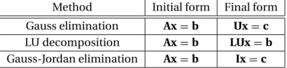
Table 2.1 lists three popular direct methods, each of which uses elementary opera-tions to produce its own final form of easy-to-solve equaopera-tions.
In the table,Urepresents an upper triangular matrix,Lis a lower triangular ma-trix, andIdenotes the identity matrix. A square matrix is calledtriangularif it con-tains only zero elements on one side of the leading diagonal. Thus, a 3×3 upper triangular matrix has the form
U= ⎡ ⎢ ⎣
U11 U12 U13
0 U22 U23
0 0 U33
⎤ ⎥ ⎦
and a 3×3 lower triangular matrix appears as
L= ⎡ ⎢ ⎣
L11 0 0
L21 L22 0 L31 L32 L33
⎤ ⎥ ⎦
Triangular matrices play an important role in linear algebra, because they sim-plify many computations. For example, consider the equationsLx=c, or
L11x1=c1
L21x1+L22x2=c2
L31x1+L32x2+L33x3=c3
If we solve the equations forward, starting with the first equation, the computations are very easy, because each equation contains only one unknown at a time. The
Method Initial form Final form
Gauss elimination Ax=b Ux=c LU decomposition Ax=b LUx=b Gauss-Jordan elimination Ax=b Ix=c
solution would thus proceed as follows:
x1=c1/L11
x2=(c2−L21x1)/L22
x3=(c3−L31x1−L32x2)/L33
This procedure is known asforward substitution. In a similar way,Ux=c, encoun-tered in Gauss elimination, can easily be solved byback substitution, which starts with the last equation and proceeds backward through the equations.
The equationsLUx=b, which are associated with LU decomposition, can also be solved quickly if we replace them with two sets of equivalent equations:Ly=b andUx=y. NowLy=bcan be solved foryby forward substitution, followed by the solution ofUx=yby means of back substitution.
The equationsIx=c, which are the produced by Gauss-Jordan elimination, are equivalent tox=c(recall the identityIx=x), so thatcis already the solution.
EXAMPLE 2.1
Determine whether the following matrix is singular:
A= ⎡ ⎢ ⎣
2.1 −0.6 1.1 3.2 4.7 −0.8 3.1 −6.5 4.1 ⎤ ⎥ ⎦
Solution Laplace’s development of the determinant (see Appendix A2) about the first row ofAyields
|A| =2.1
4.7 −0.8
−6.5 4.1
−(−0.6)
3.2 −0.8 3.1 4.1 +1.1
3.2 4.7 3.1 −6.5
=2.1(14.07)+0.6(15.60)+1.1(35.37)=0
Because the determinant is zero, the matrix is singular. It can be verified that the singularity is due to the following row dependency: (row 3)=(3×row 1)−(row 2).
EXAMPLE 2.2
Solve the equationsAx=b, where
A=
⎡ ⎢ ⎣
8 −6 2
−4 11 −7 4 −7 6 ⎤ ⎥
⎦ b=
⎡ ⎢ ⎣ 28 −40 33 ⎤ ⎥ ⎦
knowing that the LU decomposition of the coefficient matrix is (you should verify this)
A=LU= ⎡ ⎢ ⎣
2 0 0
−1 2 0 1 −1 1 ⎤ ⎥ ⎦ ⎡ ⎢ ⎣
4 −3 1 0 4 −3
0 0 2
33 2.2 Gauss Elimination Method
Solution We first solve the equationsLy=bby forward substitution:
2y1=28 y1=28/2=14
−y1+2y2= −40 y2=(−40+y1)/2=(−40+14)/2= −13 y1−y2+y3=33 y3=33−y1+y2=33−14−13=6
The solutionxis then obtained fromUx=yby back substitution:
2x3=y3 x3=y3/2=6/2=3
4x2−3x3=y2 x2=(y2+3x3)/4=[−13+3(3)]/4= −1
4x1−3x2+x3=y1 x1=(y1+3x2−x3)/4=[14+3(−1)−3]/4=2
Hence, the solution isx=2−1 3 T
.
2.2
Gauss Elimination Method
Introduction
Gauss elimination is the most familiar method for solving simultaneous equations. It consists of two parts: the elimination phase and the solution phase. As indicated in Table 2.1, the function of the elimination phase is to transform the equations into the formUx=c. The equations are then solved by back substitution. In order to illustrate the procedure, let us solve the equations
4x1−2x2+x3 =11 (a)
−2x1+4x2−2x3 = −16 (b)
x1−2x2+4x3 =17 (c)
Elimination Phase
The elimination phase utilizes only one of the elementary operations listed in Table 2.1 – multiplying one equation (say, equationj) by a constantλand subtracting it from another equation (equationi). The symbolic representation of this operation is
Eq. (i)←Eq. (i)−λ×Eq. (j) (2.6)
The equation being subtracted, namely, Eq. (j), is called thepivot equation.
We start the elimination by taking Eq. (a) to be the pivot equation and choosing the multipliersλso as to eliminatex1from Eqs. (b) and (c):
Eq. (b)←Eq. (b)−(−0.5)×Eq. (a)
After this transformation, the equations become
4x1−2x2+x3=11 (a)
3x2−1.5x3= −10.5 (b)
−1.5x2+3.75x3=14.25 (c)
This completes the first pass. Now we pick (b) as the pivot equation and eliminatex2
from (c):
Eq. (c)←Eq. (c)−(−0.5)×Eq.(b)
which yields the equations
4x1−2x2+x3 =11 (a)
3x2−1.5x3 = −10.5 (b)
3x3 =9 (c)
The elimination phase is now complete. The original equations have been replaced by equivalent equations that can be easily solved by back substitution.
As pointed out before, the augmented coefficient matrix is a more convenient instrument for performing the computations. Thus, the original equations would be written as
⎡ ⎢ ⎣
4 −2 1 11
−2 4 −2 −16 1 −2 4 17 ⎤ ⎥ ⎦
and the equivalent equations produced by the first and the second passes of Gauss elimination would appear as
⎡ ⎢ ⎣
4 −2 1 11.00 0 3 −1.5 −10.50 0 −1.5 3.75 14.25 ⎤ ⎥ ⎦
⎡ ⎢ ⎣
4 −2 1 11.0 0 3 −1.5 −10.5
0 0 3 9.0
⎤ ⎥ ⎦
It is important to note that the elementary row operation in Eq. (2.6) leaves the determinant of the coefficient matrix unchanged. This is rather fortunate, since the determinant of a triangular matrix is very easy to compute – it is the product of the diagonal elements (you can verify this quite easily). In other words,
35 2.2 Gauss Elimination Method Back Substitution Phase
The unknowns can now be computed by back substitution in the manner described in the previous section. Solving Eqs. (c), (b), and (a) in that order, we get
x3 =9/3=3
x2 =(−10.5+1.5x3)/3=[−10.5+1.5(3)]/3= −2
x1 =(11+2x2−x3)/4=[11+2(−2)−3]/4=1
Algorithm for Gauss Elimination Method
Elimination Phase
Let us look at the equations at some instant during the elimination phase. Assume that the firstk rows ofAhave already been transformed to upper-triangular form. Therefore, the current pivot equation is thekth equation, and all the equations be-low it are still to be transformed. This situation is depicted by the augmented co-efficient matrix shown next. Note that the components ofAare not the coefficients of the original equations (except for the first row), because they have been altered by the elimination procedure. The same applies to the components of the constant vectorb.
⎡ ⎢ ⎢ ⎢ ⎢ ⎢ ⎢ ⎢ ⎢ ⎢ ⎢ ⎢ ⎢ ⎢ ⎢ ⎢ ⎢ ⎢ ⎢ ⎣
A11 A12 A13 · · · A1k · · · A1j · · · A1n b1
0 A22 A23 · · · A2k · · · A2j · · · A2n b2
0 0 A33 · · · A3k · · · A3j · · · A3n b3
..
. ... ... ... ... ... ... 0 0 0 · · · Akk · · · Akj · · · Akn bk
..
. ... ... ... ... ... ... 0 0 0 · · · Aik · · · Aij · · · Ain bi
..
. ... ... ... ... ... ... 0 0 0 · · · Ank · · · Anj · · · Ann bn
⎤ ⎥ ⎥ ⎥ ⎥ ⎥ ⎥ ⎥ ⎥ ⎥ ⎥ ⎥ ⎥ ⎥ ⎥ ⎥ ⎥ ⎥ ⎥ ⎦
← pivot row
← row being transformed
Let theith row be a typical row below the pivot equation that is to be trans-formed, meaning that the elementAik is to be eliminated. We can achieve this by
multiplying the pivot row byλ=Aik/Akk and subtracting it from theith row. The
corresponding changes in theith row are
Aij ←Aij−λAkj, j =k,k+1,. . .,n (2.8a)
bi ←bi−λbk (2.8b)
i=k+1,k+2. . .,n (chooses the row to be transformed). The algorithm for the elimination phase now almost writes itself:
for k in range(0,n-1): for i in range(k+1,n):
if a[i,k] != 0.0: lam = a[i,k]/a[k,k]
a[i,k+1:n] = a[i,k+1:n] - lam*a[k,k+1:n] b[i] = b[i] - lam*b[k]
In order to avoid unnecessary operations, this algorithm departs slightly from Eqs. (2.8) in the following ways:
• IfAikhappens to be zero, the transformation of rowiis skipped.
• The indexj in Eq. (2.8a) starts withk+1 rather thank. Therefore,Aikis not
re-placed by zero, but retains its original value. As the solution phase never accesses the lower triangular portion of the coefficient matrix anyway, its contents are ir-relevant.
Back Substitution Phase
After Gauss elimination the augmented coefficient matrix has the form
A b
=
⎡ ⎢ ⎢ ⎢ ⎢ ⎢ ⎢ ⎣
A11 A12 A13 · · · A1n b1
0 A22 A<