Munich Personal RePEc Archive
Evaluation of the ocean ecosystem:
climate change modelling with backstop
technology
Tamaki, Tetsuya and Nozawa, Wataru and Managi,
Shunsuke
Urban Institute, Departments of Urban and Environmental
Engineering, School of Engineering, Kyushu University, 744
Motooka, Nishiku, Fukuoka 819-0395, Japan, Urban Institute,
Departments of Urban and Environmental Engineering, School of
Engineering, Kyushu University, 744 Motooka, Nishiku, Fukuoka
819-0395, Japan, Urban Institute, Departments of Urban and
Environmental Engineering, School of Engineering, Kyushu
University, 744 Motooka, Nishiku, Fukuoka 819-0395, Japan
31 July 2017
Online at
https://mpra.ub.uni-muenchen.de/80549/
Evaluation of the ocean ecosystem: climate change
modelling with backstop technology
Tetsuya TAMAKI
∗Wataru NOZAWA
†Shunsuke MANAGI
‡August 2, 2017
Abstract
This paper discusses the economic impacts of climate change, including those on ecosys-tems, and whether a new backstop technology should be used under conditions of strict temperature targets. Using the dynamic integrated climate-economy (DICE) model, we developed a new model to calculate the optimal path by considering new backstop technologies, such as CO2 capture and storage (CCS). We identify the effects of pa-rameter changes based on the resulting differences in CO2 leakage and sites, and we analyse the feasibility of CCS. In addition, we focus on ocean acidification and con-sider the impact on economic activity. As a result, when CCS is assumed to carry a risk of CO2 leakage and acidification is considered to result in a decrease in utility, we find that CCS can only delay the effects of climate change, but its use is necessary to achieve strict targets, such as a 1.5 ◦C limit. This observation suggests that if the
target temperature is too tight, we might end up employing a technology that sacrifices the ecosystem too greatly.
Keywords: climate change; ocean acidification; economic impact; CCS; CEEM
∗Urban Institute, Departments of Urban and Environmental Engineering, School of Engineering, Kyushu
University, 744 Motooka, Nishiku, Fukuoka 819-0395, Japan, Corresponding author: [email protected]
†Urban Institute, Departments of Urban and Environmental Engineering, School of Engineering, Kyushu
University, 744 Motooka, Nishiku, Fukuoka 819-0395, Japan
‡Urban Institute, Departments of Urban and Environmental Engineering, School of Engineering, Kyushu
1
Introduction
The possibility of global warming began to be considered near the end of the 20th century,
and global warming is now recognized as a problem throughout the world. In 1992, the
United Nations Conference on Environment and Development (UNCED) was held in Rio
de Janeiro, and the United Nations Framework Convention on Climate Change (UNFCCC)
was adopted. The Intergovernmental Panel on Climate Change (IPCC) recommended that
the average temperature increase should be kept to less than 2 degrees in the IPCC Fifth
Assessment Report (Stocker et al., 2013). Moreover, a 1.5-degree limit was cited as a target
at the 2015 United Nations Climate Change Conference (COP21) held in Paris in 2015.
The impacts of increasing temperature have been analysed by many researchers (Leemans and Eickhout,
2004; Warren et al., 2006, 2011). Recently, it has been reported that an increase in the
av-erage temperature is associated with climatic drought risks (Vicente-Serrano et al., 2014),
coastal flood risks (Hinkel et al., 2014) and human health risks (Hajat et al., 2014; Komen et al.,
2015). Parry et al. (2001) noted that the various risks increase rapidly when the
tempera-ture increase is approximately 1.5 - 2 degrees. Warren (2006) warned of the impacts of an
increasing average temperature on the ecosystem. It was suggested that a 1-degree increase
in temperature may induce a 10% ecosystem transformation and a loss in cereal production
of 20 to 35 million tons, that a 2-degree increase in temperature may induce a 97% loss of
coral reefs, and so forth. Moreover, few ecosystems may be able to adapt to an increase in
temperature of more than 3 degrees. These risks are present, and we must take measures to
rapidly mitigate or adapt to them.
In addition to evaluations of the individual risks, integrated evaluations of climate change
have been presented. Cline (1992a,b) conducted a cost-benefit analysis of climate change,
considering environmental loss, human life, disasters, water supply, and so forth. Based on
the results of this analysis, Cline concluded that an aggressive policy that would require
cut-backs of 70% of predicted emission by the middle of this century can be justified. Moreover,
of no action.
By contrast, Nordhaus took a more optimistic stance on climatic change, based on his
DICE model (Nordhaus, 1992). This model can comprehensively analyse economic impacts
while considering dynamic CO2circulation1. The model indicates that long-term, continuous
reduction of CO2 emissions is preferable to a large, abrupt reduction in the near future.
The causes of these conflicting conclusions include the magnitude of the discount rate,
the uncertainty or ambiguity of the parameters, and the irreversibility of climate change.
The conservative stance of the DICE model is often criticized. Kaufmann (1997) reported
that the DICE model contains unsupported assumptions, simple extrapolations, and
mis-specifications and that it consequently underestimates the effects of climate change. The
robustness of the DICE model with respect to ambiguity was assessed by Hu et al. (2012).
Hu et al. observed that the ineffectiveness noted by Nordhaus is significantly increased when
the ambiguity of distribution is considered but insisted that a lack of any emission control
policies may carry a high risk and doing nothing is by no means a rational response. Other
researchers have extended the DICE model in various directions to achieve greater realism.
For example, De Bruin et al. (2009) developed the AD-DICE model by introducing
adapta-tion as another control variable. The AD-DICE model can estimate the adaptaadapta-tion costs
of climate change by splitting the net damages into residual damages and protection costs.
The ENTICE model developed by Popp (2004, 2006) separates energy units from inputs and
treats technological change as an endogenous variable. The uncertainty in the DICE model
with regard to the level of damage caused by global warming was also analysed by Traeger
(2014) and Crost and Traeger (2014). In addition to the DICE model, various other
Inte-grated Assessment Models (IAMs) have also been developed. The features of these models
have been summarized by Dowlatabadi (1995); Stanton et al. (2009).
These models, such as the DICE model, are classified among the welfare optimization
type. Nevertheless, many IAMs use other methodologies; general equilibrium(Gerlagh, 2008),
1
simulation (Dowlatabadi, 1998; Hinkel, 2005; Hope, 2006) and so forth. Welfare optimization
models are simple yet transparent, making them suitable for the analysis of conceptual
models. In addition, CCS technology investment is evaluated by using real option approach
(Zhou et al., 2010; Zhu and Fan, 2011). Also CCS had been introduced to some
energy-economic system models (Syri et al., 2008; Held et al., 2009).
This study focuses on the impact on ecosystems or the environment. The DICE model
assumes that the technological costs of emission reduction will be reduced in the future by
virtue of technical innovations. This assumption is not unsupportable, but new technologies
will not necessarily bring only benefits. Some new technologies may carry unknown risks.
For example, a mitigation technique known as CO2 capture and storage (CCS) has recently
been attracting attention. CCS is a method based on capturing waste CO2, such as that
from power plants, and transporting it to deep underground storage areas. According to
Metz et al. (2005), CCS could reduce global emissions by 9-12% by 2020 and 21-45% by
2050. The GlobalCCSInstitute (2016) reports that in sectors with high-concentration gas
streams (natural gas processing sector, ammonia/fertiliser production sector, bio-ethanol
production sector, hydrogen production sector, iron and steel production sector), large-scale
CO2 capture projects are underway. Three principal types of capture technologies are used;
pre-combustion, oxyfuel combustion, and post-combustion. These technologies have been
analysed, and their impacts and efficiencies were reported (Koornneef et al., 2008; Li et al.,
2009; Park et al., 2011). The optimal technology is selected and implemented according to
the physical properties of CO2 emitted from each emission source across several industries.
For example, post-combustion technology is used to capture CO2 in the cement industry
(Cormos and Cormos, 2017), and with pre-combustion being used in industrial processes,
such as natural gas(Kanniche et al., 2010) and oil (Weydahl et al., 2013). In addition, the
technology of bio-energy with carbon capture and storage (BECCS)(Azar et al., 2010), which
combines CCS technology in biomass power plants or biofuel manufacturing processes, has
have been assessed by many researchers(Moreira et al., 2016; Bui et al., 2017). Chemical
looping combustion process and calcium looping process have also been developed in recent
years. These technologies have, potentially, much lower cost and much higher efficiency than
other technologies (Lyngfelt et al., 2001; Fan et al., 2008; Zhu et al., 2015; Perej´on et al.,
2016). 2
However, some researchers are concerned about the possibility of CO2 leakage. Such
leakage may cause local ocean acidification (Blackford et al., 2009) and may impact the
biodiversity of marine life (Kroeker et al., 2013). Currently, CCS is still expensive, but
its cost is expected to decrease to a feasible level in the future. At that time, it will be
necessary to decide whether to adopt this technology. To determine the best among the
possible technologies, it will be important to assess the effects that we may suffer from their
unknown risks. Efforts have been made to perform comprehensive evaluations of CCS at
the plant and macroeconomic levels (Viebahn et al., 2012, 2014, 2015; Pettinau et al., 2017;
Sathre et al., 2012; Koelbl et al., 2016).
Moreover, we cannot overlook the potential damage to the ecosystem. Although we do
not have a detailed picture of the services provided by the ecosystem and their value because
of the complexity and vastness of the ecosystem, many researchers have presented estimates.
For example, the value of ecosystem services as estimated by Costanza et al. (1997) and
Balmford et al. (2002) is in the range of US$ 16 - 54 trillion per year. Focusing on commercial
value, Narita et al. (2012) reported that the global economic costs of mollusc loss from ocean
acidification may be more than US$ 100 billion if the mollusc demand increases with future
income rise.
With these studies in mind, we attempt to determine whether technologies that reduce
CO2 but carry ecosystem pollution risks should be used under conditions of strict
tempera-ture targets. To address this question, we modify the DICE model accordingly and analyse
the temperature targets. The three main contributions of this study can be summarized as
2
follows. The first contribution is a modification of the DICE model. By addressing several
backstop technologies, we consider the possible effects of introducing technologies such as
CCS. We show that the optimal choice of whether CCS should be used changes depending
on the leakage ratio and the leakage sites. The second contribution is a consideration of
the fact that if more people begin to feel that ocean acidification will result in a decrease in
utility, then the optimal level of emission should be considerably less. This effect may result
in a 0.5-degree decrease in the desired average temperature even if the direct effect on utility
caused by acidification is less than 1% with respect to the consumption utility. The negative
impacts of ocean acidification caused by CO2 leakage have been recognized, and local
im-pacts have been intensively investigated in laboratory-based, field, and natural experiments
(Widdicombe and Spicer, 2008; Widdicombe et al., 2013; Murray et al., 2013; Ishida et al.,
2013). The novelty of our work lies in providing an assessment of the potential of CCS
as a mitigation technology at the global level, based on those seminal experimental works.
Models that focus on CCS use have previously been developed (Mori, 2012; Lee, 2017), but
these models do not consider ecosystem damage. Finally, we address policies that call for a
2-degree target and a 1.5-degree target. As discussed by Azar et al. (2006) and Scott et al.
(2013), CCS is regarded as a core component of emission-reduction scenarios, and thus, it
is important to evaluate the potential of CCS for reaching degree targets (Tollefson, 2015).
Previous studies in this context include those of Azar et al. (2010) and Selosse and Ricci
(2017). We contribute to the literature by explicitly modelling the negative impact of CO2
leakage into the ocean and examining the simulated optimal plan at the global level. The
results of our simulation analysis show that these targets are rather strict, and the social cost
of carbon (SCC) becomes quite high in comparison with the optimal control case. However,
if we must implement such a strict target, we will be required to use lower-cost technologies
despite their potential risk to the environment.
This paper is structured as follows. Section 2 presents the DICE model and its theoretical
climate-ecosystem-economy model (CEEM), introducing a backstop technology that can
capture and store CO2 but carries a risk of leakage into the atmosphere and ocean. We
consider the harmful effects of this leakage from the perspective of ocean acidification in
section 4, and we explore how the optimal solution is affected. Moreover, we analyse the
2-degree and 1.5-degree targets using our model. The last section presents our conclusions.
2
DICE model
Our model, the CEEM, is based on the DICE model. Therefore, we introduce the DICE
model in detail in this section, and we describe the additional features (consideration of
additional backstop technologies and the ocean ecosystem) incorporated into the CEEM in
the following section.
The DICE model is a dynamic optimization model for analysing the effects of climate
change. This model is primarily based on the Ramsey model, and the total utility to be
maximized is represented by the following expression:
T ∑
t=1
U[c(t), L(t)] (1 +ρ)−t, (1)
U[c(t), L(t)] =L(t)[c(t)]
1−α
1−α ,
whereU is the utility,L(t) is the labour in time period t,c(t) is the flow of consumption per
capita in periodt,ρis the discount rate and is assumed to be 0.3, andαis the elasticity of
in-tertemporal substitution and is assumed to be 1.45. This optimization problem includes two
sets of constraints: one represents economic constraints, and the other represents emission
2.1
Economic constraints
First, let us consider the economic constraints. IfA(t),K(t) andL(t) denote the total factor
productivity (TFP), capital and population, respectively, in period t, then the production
Q(t) is given by
Q(t) = Qnet(t)−Λ(t)A(t)K(t)γL(t)1−γ, (2)
Qnet(t) =A(t)K(t)γL(t)1−γ[1−Ω(t)], (3)
whereγ is the elasticity of output with respect to capital and is assumed to be 0.3 and Λ(t)
and Ω(t) are the abatement cost ratio and the climate damage ratio, respectively. These two
variables are given by
Λ(t) = θ1(t)p(t)µ(t)θ2, (4)
Ω(t) = ψ1TAT(t) +ψ2[TAT(t)]2. (5)
The abatement cost ratio, Λ(t), represents the cost of emission reduction as determined by
the emission control rate µ(t). p(t) is the cost of the backstop technology, and θ1(t) and
θ2 are parameters. θ1 and θ2 are assumed to be defined by the equation θ1(t) =σ(t)/2800
and to be equal to 2.8, respectively. Here, σ(t) is the level of carbon intensity (mentioned
below). The abatement cost is calculated based on the assumption that it is proportional to a
power function of the reduction rate. Meanwhile, the climate damage ratio Ω(t) is expressed
as a quadratic function of the atmospheric temperature TAT(t) and the parameters ψ1 and
ψ2. Tol (2009) estimated that a 3 ◦C increase in temperature will cause damage equivalent
to approximately 3% of the global output. However, this estimate ignores several factors,
such as biodiversity, ocean acidification and sea level rise. Therefore, Nordhaus and Sztorc
(2013) set the parameter values to ψ1 = 0.00267 and ψ2 = 2 to include additional damage
This extent of damage is supported by Anthoff and Tol (2010) and Hope (2011). The TFP,
A(t), and the population growth, L(t), are exogenous. These quantities take the forms
A(t+ 1) =A(t) [1 +gA(t)],
L(t+ 1) =L(t) [pop/L(t)]padj,
where gA(t) = 0.079·e−δA·t and δA, pop, and padj represent the rate of decline of the TFP,
the future population, and the rate of population growth, respectively. The values of these
three parameters are assumed to be 0.03, 10500, and 0.134, respectively. The gross output,
Q(t), is divided into a consumption term, C(t), and an investment term, I(t):
Q(t) =C(t) +I(t).
In this model, the per capita consumption is defined as
c(t) = C(t) L(t).
Finally, the capital stock, K(t), is given by
K(t) = I(t)−δKK(t−1),
where δK is the capital depreciation rate and has a value of 0.1.
2.2
Emission and carbon cycle constraints
The original DICE model considers the carbon cycle. Concretely, the carbon cycle as
mod-elled in the original DICE model consists of three layers: the atmosphere, the upper ocean
and the deep ocean. In addition, countries release CO2 from production activities in
These CO2 emissions circulate through the three layers of the model.
A country’s total emission E(t) is given by
E(t) = EInd(t) +ELand(t),
where EInd(t) represents the emission from the country’s production activities and ELand(t)
represents its emissions related to land use. The corresponding equations are
EInd(t) = σ(t) [1−µ(t)]A(t)K(t)γL(t)1−γ,
ELand(t) = eland0×(1−deland)t−1,
whereσ(t) is the level of carbon intensity,eland0 is the amount of CO2from land use released
in 2010, and delandis the rate of decline of land use emissions. Nordhaus and Sztorc (2013)
assumed thatσ(t) is given byσ(t+ 1) =σ(t)·egσ(t)
, withgσ(t+ 1) = 1.001·gσ(t). ELand(t) is
an exogenous value, andeland0 anddelandare assumed to be 3.3 and 0.2, respectively. The
DICE model assumes three reservoirs of carbon: the amount of carbon in the atmosphere
is denoted by MAT(t), that in the upper ocean is denoted by MU P(t), and that in the deep
ocean is denoted by MLO(t). The equations describing the carbon cycle are as follows:
MAT(t) = E(t) +φ11MAT(t−1) +φ21MU P(t−1),
MU P(t) = φ12MAT(t−1) +φ22MU P(t−1) +φ32MLO(t−1), (6)
MLO(t) = φ23MU P(t−1) +φ33MLO(t−1).
The coefficientsφij are parameters representing the flow from reservoir ito reservoir j 3.
Nordhaus set these parameters as constants in his three-reservoir model. The accumulation
of CO2 causes global warming as a result of increases in radiative forcing. This model follows
3
the original DICE model:
F(t) = ηlog2 MAT(t) MAT(1750)
+FEX(t),
where F(t) is the change in the total radiative forcing caused by GHGs from anthropogenic
sources, such as CO2, since 1750. FEX(t) represents exogenous forcing 4, and η is an
ad-justable parameter that is assumed to have a value of 3.8. Moreover, the air temperature
and the deep ocean temperature are defined as follows:
TAT(t) = TAT(t−1)+ξ1{F(t)−ξ2TAT(t−1)−ξ3[TAT(t−1)−TLO(t−1)]},
TLO(t) = TLO(t−1) +ξ4[TAT(t−1)−TLO(t−1)],
where ξ1 = 0.098, ξ2 = 1.31, ξ3 = 0.088, and ξ4 = 0.025. These equations are explained in
detail in the manual for the DICE model (Nordhaus and Sztorc, 2013). The main parameters
are listed in the Appendix. For actual calculations using the DICE model, the time step is
chosen to be 5 years, 60 time periods (300 years) are assumed, and the initial values are as
shown in Table 1.
Table 1: Initial conditions
A(1) L(1) Q(1) K(1) µ(1) E(1) σ(1)
[mil.] [$tril.] [$tril.] [GtCO2/yr]
3.8 6838 63.69 135 0.039 33.61 0.549
4
FEX(t) is assumed to obey the following equation: FEX(t) =
{
3
New backstop technology
We formulate a new model, the CEEM, by adding two new features to the DICE model:
an additional kind of backstop technology and the ocean ecosystem. As discussed later, the
addition of these features leads to crucial changes in the optimal solution and the evaluation
of the 2-degree and 1.5-degree targets.
3.1
Modelling of two backstop technologies
The cost of a backstop technology in the DICE model is given as follows:
p(t) =pback(1−gback)t−1, (7)
where pback is the initial cost ($/tCO2) of the backstop technology and gback is the rate
of decline of this cost. p(t) is a decreasing function, and the abatement cost ratio, Λ(t),
decreases as p(t) decreases. Thus, the rate of emission reduction, µ(t), will readily increase
as time goes on.
The costs for backstop technologies based on renewable energy, such as solar power, and
other technologies will be lower in the future, but not all such technologies are safe for the
environment. The impacts of CCS, for example, have not yet been sufficiently explored.
Therefore, this study suggests the modelling of two kinds of backstop technologies: one is
the type of technology supported by the DICE model, and the other is a technology that
can exert undesirable effects on the environment. We refer to these types of technologies
as conventional backstop technology (BT1) and CCS-type backstop technology (BT2). The
corresponding costs, in analogy to Eq. (7), are given as follows:
p1(t) =pback1(1−gback1)t−1,
Letx(t) be the rate of BT2 use; then, Eq. (4) becomes
Λ(t) = θ1(t){[1−x(t)]p1(t) +x(t)p2(t)}µ(t)θ2.
Hence, the emission reduction achieved by means of BT2, EBT2(t), is given by
EBT2(t) = σ(t)µ(t)x(t)A(t)K(t)γL(t)1−γ.
A BT2 technology, such as CCS, carries a risk of CO2 leakage into the ocean or the
atmo-sphere, which may cause an increase not only in temperature but also in ocean acidification.
To analyse the impact of this risk, we define V(t) as the amount of BT2 storage in time
period t:
V(t+ 1) = [1−l(t)]V(t) +EBT2(t),
where l(t) is the leakage rate in period t and is specified exogenously. Then, for example,
when we assume that the leakage occurs into the atmosphere and upper ocean, Eq. (6)
becomes
MAT(t) = E(t) +φ11MAT(t−1) +φ21MU P(t−1) +k·l(t)V(t),
MU P(t) = φ12MAT(t−1) +φ22MU P(t−1) +φ32MLO(t−1) + (1−k)l(t)V(t), (8)
MLO(t) = φ23MU P(t−1) +φ33MLO(t−1),
wherekis the rate of leakage into the atmosphere. It can be interpreted as being determined
3.2
Backstop technologies and the optimal strategy
In this section, we demonstrate the effects of varying the rate and sites of leakage on the
opti-mal solution. We compute the optiopti-mal solution under three different assumptions regarding
the leakage rate l(t): (i) the leakage is constant over time, l(t) = 0.02; (ii) the leakage is
increasing at a low rate, l(t) = 0.01·1.01t−1−0.01; and (iii) the leakage is increasing at a
high rate, l(t) = 0.01·1.05t−1−0.01. As mentioned by Widdicombe et al. (2013), the risk
of leakage is a matter of concern. The leakage itself is uncertain, and the level of risk is not
well known. Hence, to be conservative, we assume that the leakage is certain and investigate
whether BT2 should be used or not under this assumption.
First, we consider the case of leakage only into the upper ocean, namely, k = 0 in Eq.
(8). The initial cost of BT1, pback1, is chosen to be 344 ($/tCO2), the same as in the
DICE model, version 2013R. As discussed above, BT2 is assumed to be an inferior type of
technology compared with BT1 because BT2 involves leakage. Therefore, if BT2 is more
expensive than BT1, BT2 will never be used at all. Accordingly, we set the initial cost of
BT2 to 300, which is lower than that of BT1; this particular value is chosen for convenience.
Table 2 summarizes the parameters related to the backstop technologies.
Table 2: Parameters related to backstop technologies
parameter
pi(t) the cost of backstop technology i in time period t (i= 1,2)
pbacki the initial cost of backstop technology i (i= 1,2)
gbacki the rate of decline of the cost of backstop technology i (i= 1,2)
l(t) the leakage rate in time periodt
k the leakage rate into the atmosphere
variable
x(t) the rate of BT2 use
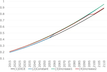
Figure 1 and Figure 2 illustrate the carbon emissions and the emission control rates,
respectively, under the various leakage conditions. The solid lines represent the original
Figure 1: Total carbon emission
Note: (1) Original DICE model. (2) Constant leakage: l(t) = 0.02. (3) Increasing leakage: l(t) = 0.01·1.01t−1−0.01. (4) Increasing leakage: l(t) = 0.01·1.05t−1−0.01.
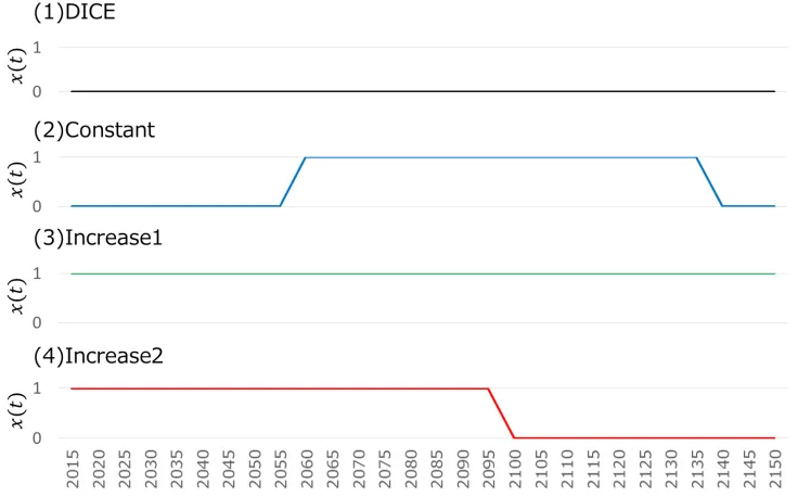
[image:16.612.123.492.418.669.2]Figure 3: Backstop technology utilization
different leakage rates. By comparing the DICE model with the other settings, we can see
that emissions are reduced when BT2 is available. The dashed lines, which represent the three
settings with BT2, show different patterns of both the total carbon emission and the emission
control rate. To elucidate the mechanism behind these patterns, let us consider Figure 3,
which illustrates the utilization of the backstop technologies. We find that differences in
the relative rates of use of these technologies arise from the different leakage conditions,
and the levels of emission differ considerably depending on the situation. In particular, we
note that the timings of the introduction and discontinuation of the different technologies
change depending on the leakage situation. For example, if the leakage rate is constant (e.g.,
l(t) = 0.02), then we should not introduce BT2 until approximately 2060 and should stop
using BT2 in approximately 2140. By contrast, if the leakage rate is exponentially increasing
(e.g., l(t) = 0.01·1.05t−1−0.01), then we would be better served to introduce BT2 as soon
as possible. Note that the utilization differs depending on the initial cost, the leakage rate,
the cost decline rate, and other parameters.
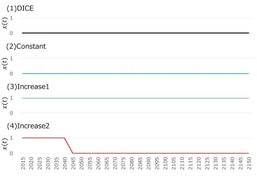
leakage sites. In the above analysis, we assume that leakage occurs only into the upper ocean,
but there is a possibility that leakage may occur not only into the ocean but also near the
ground. This would further accelerate the elevation of the atmospheric temperature. Figure
4 illustrates the utilization situation of the backstop technologies in the case of k= 0.2. The
other parameters are the same as in the above analysis. By comparing the different possible
leakage locations, we can see that BT2 is difficult to use at all in the case of leakage into the
atmosphere and ocean; a comparison of Figure 3 and Figure 4 shows that when the leakage
rate isl(t) = 0.2 orl(t) = 0.01·1.05t−1−0.01, BT2 falls out of favour compared with the case
of k = 0. For the leakage case corresponding to l(t) = 0.01·1.01t−1 −0.01, the utilization
does not change with variations in the parameter k. The reason for this must be that the
absolute amount of leakage in the case of l(t) = 0.01·1.01t−1 −0.01 is smaller than in the
[image:18.612.122.490.358.610.2]other cases.
Figure 4: Backstop technology utilization for k= 0.2
From these results, we can see that introducing new technologies is of great worth even
of low leakage into the atmosphere. However, we should note that leakage into the ocean
will cause acidification and may damage the ocean ecosystem.
4
Ocean ecosystem
4.1
Framework for including ecosystem damage
Next, we consider the impact on the ocean ecosystem. The leakage of CO2 from storage areas
may cause not only an increase in temperature but also environmental damage, such as ocean
acidification. This acidification will exert undesirable effects on the ocean ecosystem, e.g.,
inhibition of the growth of shellfish.
The ocean ecosystem provides several kinds of services (Barbier et al., 2011). Damage to
the ocean ecosystem caused by acidification will eventually cause damage to the economy.
As described above (section 2.1), the damage function given in Eq. (5) already considers
the economic damage to the ocean ecosystem. However, there are expected to be
addi-tional factors that would be difficult to convert into economic costs. Based on their survey,
Adams and Adger (2013) suggested that the well-being of the ecosystem is of considerable
importance. Although, in general, many researchers use consumption as the only variable in
the utility function, there is some disagreement regarding this approach. Jones and Klenow
(2016) suggested that the utility function should include not only consumption but also
leisure, mortality, and inequality, whereas Grimaud and Rouge (2008) defined the utility as
a function of consumption and environment stock in their model. Hence, we use the utility
function defined as follows.
This study demonstrates the effect of introducing an acidification index, such as pH, into
gas in the upper ocean; then, the pH is given by
pH(t) = pK−logZ(t)
2 ,
Z(t) = MU P(t)
ζ ,
where pK is the dissociation constant andζ is an adjustment parameter. Then, we assume
that damage to the ecosystem results in a decrease in utility. Let G(t) be the decrease in
utility caused by a change to the level of ocean acidification; then,
G(t) = [pH(t)−pH(0)]2, (9)
under the assumption that the economic loss due to a deviation of the pH from its initial
level grows quadratically. Consequently, Eq. (1) becomes
T ∑
t=1
{U[c(t), L(t)]−ωG(t)}(1 +ρ)−t, (10)
where ω is a damage parameter. Note that these functional forms and parameters are not
supported by quantitative empirical evidence. Consequently, the outcomes of the model
should not be treated as quantitatively accurate, only qualitatively.
4.2
Results of the CEEM
First, the acidification parameters are set as follows. Although measurements of pH in the
ocean are not straightforward, the pH values typically range from 7.7 to 8.2 (Brewer et al.,
1995). Based on these values, we assume that the initial pH value pH(0), pK and ζ are
8.21, 6.5 and 2.42×10⁷, respectively. With these values, in the original DICE model, thepH
value becomes 8 or 7.9 when the atmospheric temperature increases by approximately 2.3
degrees or 3.3 degrees, respectively. These predictions are not inconsistent with estimations
have noted the possibility of a reduction in pH by 0.2 - 0.5 units over the next century.
The degree of ocean acidification is directly affected by the amount of carbon in the upper
ocean,MU P, in this model. Depending on whether leakage occurs only into the ocean (k = 0)
or into both the atmosphere and the ocean (k > 0), the resulting level of acidification differs.
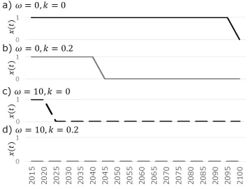
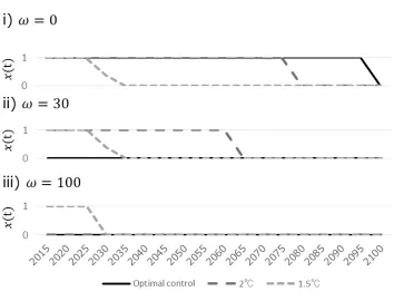
Figure 5 shows the backstop technology utilizationx(t) for the leakage scenario characterized
byl(t) = 0.01·1.05t−1−0.01 for four pairs of values of the parameter representing the utility
loss caused by acidification, ω, and the parameter representing the rate of leakage into the
atmosphere, k: (ω, k) = (0,0), (0,0.2), (10,0) and (10,0.2). First, let us compare the first
two cases, (ω, k) = (0,0) and (ω, k) = (0,0.2). We find that BT2 is used less often in the
case of leakage into both the atmosphere and the ocean (k= 0.2) compared with leakage into
only the ocean (k = 0). This trend does not change even when acidification is considered
to cause a decrease in utility (ω = 10). The effect of a change in the damage parameter
is quite intuitive. A comparison between the two cases with ω = 0 and the two cases with
ω = 10 shows that the decrease in utility caused by acidification results in a decrease in
BT2 utilization. In other words, when the value of the damage parameter ω is higher, CO2
leakage is more undesirable.
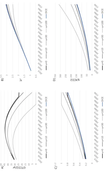
Let us explore the effect of the damage parameterω in greater detail. Figure 6 shows the
results of optimal control for four levels of the damage parameterω: 0, 10, 30, and 100. The
parameter describing the leakage into the atmosphere, k, is set equal to 0 in this exercise. A
higher level of the parameterω leads to higher emission control rates, as depicted in Figure
6-(C). Because of the change in the emission control rate, industrial emissions are reduced,
and the elevation of the temperature of the atmosphere is also suppressed. In the case of
ω = 100, the atmospheric temperature in 2100 is 0.5 degrees lower than in the case ofω = 0,
and the social cost of carbon is approximately two times higher than in the case of ω= 0.
In both the DICE model and the CEEM, we maximize the total utility (see Eq. (1) and
Eq. (10)). The introduction of the parameter ω represents the reduction in the total utility
the utility in 2010 as the reference point and set it equal to 0. As the value ofωincreases, the
disutility due to acidification also increases. Note that the disutility due to acidification is
less than 1% of the consumption utility in this analysis. In addition, the consumption utility
decreases asωincreases. It appears that the reason for this relationship is the increase in the
emission control rate. Although the increase in the emission control rate has a suppressing
effect on the consumption utility, the disutility due to acidification is also suppressed. A key
observation is that although the direct effect on the total utility caused by acidification is
[image:22.612.127.485.272.543.2]not large, it can cause a material change in the optimal strategy.
Figure 5: Backstop technology utilization considering ocean acidification
Figure 6: Optimal control for various values of the damage parameter ω
Table 3: Changes in utility with variations in the parameterω
Utility 2015 2020 2030 2050 2070 2090
ω= 0 Consumption 39.3 78.4 153.6 284.6 386.1 462.2
Acidification 0 0 0 0 0 0
ω= 10 Consumption 39.2 78.3 153.5 284.4 385.8 461.8
Acidification 0 0 -0.1 -0.2 -0.3 -0.5
ω= 30 Consumption 39.1 78.1 153.2 283.9 385.2 461.2
Acidification 0 -0.1 -0.2 -0.5 -0.9 -1.3
ω= 100 Consumption 38.8 77.5 152.3 282.4 383.2 460
Acidification -0.1 -0.3 -0.6 -1.5 -2.6 -3.7
Note: These utility values represent the increase (or decrease) with respect to the utility in 2010. The consumption utility and the acidification utility correspond toU(·) and ωG(t), respectively.
4.3
2-degree target and 1.5-degree target
Here, let us consider a 2-degree target and a 1.5-degree target. A 2-degree target was adopted
in the Copenhagen Accord, and this target has been referenced at various international
con-ferences. Moreover, a stricter 1.5-degree target has become a focus since COP21. Nordhaus
(2014) estimated the social cost of carbon (SCC) in the context of the 2-degree target using
the DICE model, version 2013R, and found that the SCC rises sharply.
In this section, we compare the results of the DICE model and the CEEM model when
evaluating the 2-degree target and the 1.5-degree target. We assume that the leakage is
characterized by l(t) = 0.01·1.05t−1 −0.01 and k = 0. For the damage parameter ω, we
use three values: 0, 30, and 100. Table 4 shows the estimated SCC values. In the case of
the DICE model, the SCC values for the 2-degree case are 47.6, 216.4 and 561.8 ($/tCO2)
in 2015, 2050 and 2090, respectively. These are approximately 2.6, 4.1 and 4.7 times the
SCC values for the baseline case. In the case of the CEEM with ω = 0, meanwhile, the
SCC values for the 2-degree case are 43.9, 199.2 and 790.4 ($/tCO2) in 2015, 2050 and 2090,
respectively. These are approximately 2.4, 3.7 and 6.6 times the SCC values for the baseline
case. The SCCs obtained using the CEEM are lower than those from the DICE model in
model in the far future. This behaviour seems to be due to the influence of BT2. BT2 can
store CO2, but the stored CO2 is assumed to gradually leak in this model. This means that
current emissions are suppressed at the cost of increased emissions in the far future. Hence,
we can achieve a lower SCC in the near future, but the problem will come back to haunt us
in the far future.
Next, we focus on the case of the 1.5-degree target. We find that the SCC increases
considerably compared with the SCC values in the cases of the baseline, the optimal control
strategy, and the 2-degree target, as shown in Table 4. The values for the 1.5-degree case
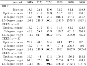
are more than 10 times those for the baseline case. Figure 7 presents the ratio of the SCC
values between the DICE and CEEM evaluations. This ratio increases more slowly under
the 1.5-degree target than it does under the 2-degree target. For example, the SCC in 2100
that is indicated by the CEEM with ω = 30 is 1.4 times that indicated by the DICE model
in the case of the 1.5-degree target, whereas it is 2.2 times that indicated by the DICE
model in the case of the 2-degree target. By contrast, between 2050 and 2080, the ratio is
approximately 1 in both cases, although the ratio for the 2-degree case is slightly lower than
that for the 1.5-degree case until approximately 2075. Furthermore, the ratio approaches 1
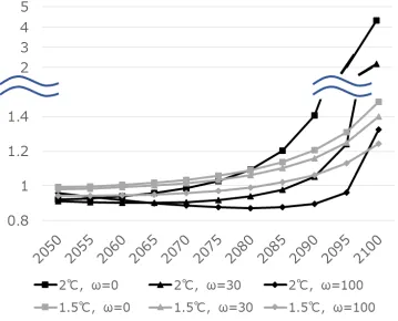
as the parameter ω increases. As shown in Figure 8, BS2 is also increasingly rarely used as
the parameter ω increases. From these results, we find that the use of BT2 postpones the
impact of climate change. In addition, forω= 100, BT2 is used only until 2035 in the case of
the 1.5-degree target and is not used at all in the case of the 2-degree target. Consequently,
the difference between the DICE and CEEM results is relatively small.
Figure 9 illustrates the change in the emission control rate. The rates for the 2-degree
target and the 1.5-degree target are little affected by increasing ω, unlike in the optimal
control case. The rate reaches 1 in either 2060 or 2030 for the case of the 2-degree target or the
1.5-degree target, respectively, regardless of any increase in ω. That is, under both targets,
an enormous amount of CO2 emissions must be processed using backstop technologies in
eliminating the majority of emissions within the next few years. In addition, in the case
of the adoption of a strict target, the index representing the level of ocean acidification as
expressed in Eq. (9) takes on a smaller value compared with the other cases. Namely, the
decrease in utility caused by acidification,ωG(t) (in Eq. (10)), is not as large as in the cases
of the other, less strict targets. Consequently, the influence of increasing ω is reduced as the
target becomes more strict. The cost of a backstop technology is defined as a decreasing
function over time, such that using BS2 earlier results in a larger benefit than using it later.
In the case of the 1.5-degree target, the benefit of using BT2 exceeds the cost of the leakage
because of the enormous amount of emissions that must be eliminated. As a result, BT2 is
used only during a short period of the early stage regardless of the value of ω. By contrast,
in the case of the 2-degree target, because the required emission reduction is not as large as
in the case of the 1.5-degree target, the usage of BT2 does depend onω, as shown in Figure
8.
Our work assesses the potential of CCS as a mitigation technology at the global level,
based on previous experimental studies. From our results, we can say that if we hope to
achieve a strict target (such as 1.5-degree target), technologies that reduce CO2 emissions
but carry a risk of ecosystem damage may be useful for reaching that target. In particular, in
this model, we assume that these new technologies are certain to result in the leakage of CO2.
Therefore, these new technologies should be used to a greater extent if the actual probability
of leakage is low. In addition, note that the optimal use of these new technologies will change
with the magnitude of the utility from the ecosystem, but in the case of the adoption of a
strict target, we may be more willing to accept the utility decrease due to ecosystem damage.
Ecosystem damage will already be reduced by achieving such a strict target, so there is a
Table 4: Social costs of carbon under the DICE model and the CEEM ($/tCO2)
Scenario 2015 2020 2030 2050 2070 2090
DICE
Baseline 18.6 22.1 30.6 53.2 83.1 119.8
Optimal control 17.7 21.2 29.3 51.5 81.9 120.6
2-degree target 47.6 60.1 94.4 216.4 437.2 561.8
1.5-degree target 196.2 249.3 406.4 1080.5 2576.3 4833.1
CEEM ω= 0
Optimal control 17.7 21.2 29.4 51.7 82.7 122.3
2-degree target 43.9 55.2 86.3 199.2 431.5 790.4
1.5-degree target 194.7 247.1 402.2 1072.1 2668.9 5824
CEEM ω= 30
Optimal control 23.7 28.3 39.4 70.1 112.9 167.8
2-degree target 46.2 57.7 88.7 197.2 396.8 592
1.5-degree target 194.8 246.9 400.5 1061 2617.9 5605.6
CEEM ω= 100
Optimal control 36.9 44 61.3 109.3 176.2 263.1
2-degree target 54.8 67.3 100.1 207.6 387.7 503.7
1.5-degree target 193.5 244 391.3 1020.2 2472.4 5137.6
Figure 8: Backstop technology utilization for various values of the parameter ω
[image:29.612.125.485.491.641.2]5
Conclusion
This paper examines the role of CCS technologies in combating climate change. In particular,
we attempt to judge whether new technologies that offer reasonable CO2 control but carry a
risk of ecosystem damage should be used under the 2- and 1.5-degree targets. Although the
CCS-type technologies that we model can capture CO2 and delay climate change, they are
known to present the possibility of leakage and harmful effects on the ecosystem. To capture
this trade-off, we established an evaluation framework that considers two types of backstop
technologies (BT1 and BT2) and the ocean ecosystem. Using this framework, we explored
the optimal solution and other policy plans, such as 2- and 1.5-degree targets.
First, we explored the optimal use of BT2 in a simple setting without any harmful
effects of BT2 on ocean acidification. We found two intuitive tendencies: (i) when the
leakage rate is lower, BT2 is used more extensively, and (ii) when more leakage goes into the
atmosphere, BT2 is used less extensively. The second relationship holds because leakage into
the atmosphere causes the atmospheric temperature to increase more quickly than leakage
into the ocean does. Interestingly, we also observed that a delay in beginning the use of BT2
is sometimes optimal.
Next, in a setting in which the harmful effects of BT2 on the ocean ecosystem are
consid-ered, we examined the optimal use of BT2 for various values of the parameter that determines
the economic cost of acidification, ω. Here, we found that when acidification is regarded as
more costly, BT2 is used to a lesser extent because the leakage becomes more costly and
overshadows the benefit of the low implementation cost. Depending on the value of ω, the
resulting increase in the atmospheric temperature by the end of this century was found to
vary from 2.5 to 3 degrees, with the impact on the utility level remaining below 1%.
Under the 2- and 1.5-degree targets, we found a different pattern. In contrast to the
case of the optimal solution (with no temperature target), varying the economic cost of
acidification,ω, does not strongly impact the optimal plan under the 2- or 1.5-degree target.
target, an enormous amount of emissions must be eliminated early on, and consequently, the
cost advantage of BT2 is valued more highly. The other is that if we adopt a strict target, the
index representing the level of ocean acidification (G(t)) becomes smaller than in the case of
a laxer target. As a result, the term expressing the decrease in utility caused by acidification,
ωG(t), does not become as large with increasing ω as it does for laxer targets. In the case
of the largest considered ω value, BT2 is used only in the case of the 1.5-degree target. In
the optimal solution, BT1 is always employed, and BT2 is never used. This observation tells
us that if we adopt a target temperature that is too tight, we might end up employing a
technology that sacrifices the ecosystem too greatly.
Finally, we considered the SCC. The SCC in the case of the 2-degree target is much
higher than that in the optimal control case, and the SCC in the case of the 1.5-degree
target is even higher than that under the 2-degree target. The difference between the DICE
and CEEM evaluations becomes increasingly large in the far future because of the use of
BT2. We found that by using BT2, we can keep the SCC at a lower value in the near future,
but this comes at the cost of a greater increase in the far future. However, the difference
between the DICE model and the CEEM becomes small as the value of the parameter ω
increases. This is because BS2 is rarely used at higher values of ω because of the enormous
cost of acidification.
Nomenclature
BECCS bio-energy with CO2 capture and storage
BT1 conventional backstop technology
BT2 CCS-type backstop technology
CCS CO2 capture and storage
COP21 2015 United Nations Climate Change Conference
GHGs greenhouse gases
IP CC Intergovernmental Panel on Climate Change
SCC social cost of carbon
T F P total factor productivity
U N CED United Nations Conference on Environment and Development
U N F CCC United Nations Framework Convention on Climate Change
Models
AD−DICE adaptation in DICE
CEEM dynamic integrated climate-ecosystem-economy model
DICE dynamic integrated climate-economy
EN T ICE endogenous technological change in DICE
IAM s integrated assessment models
Acknowledgements
Financial support for this work was provided by the Environment Research and Technology
Development Fund (S-14) of the Ministry of the Environment of Japan and by Specially
Promoted Research through a Grant-in-Aid (Scientific Research 26000001) from the Japanese
Ministry of Education, Culture, Sports, Science and Technology (MEXT).
References
mak-ing on climate change. Journal of Environmental Economics and Management, 60(1):14– 20.
Azar, C., Lindgren, K., Larson, E., and M¨ollersten, K. (2006). Carbon capture and stor-age from fossil fuels and biomass–costs and potential role in stabilizing the atmosphere.
Climatic Change, 74(1):47–79.
Azar, C., Lindgren, K., Obersteiner, M., Riahi, K., van Vuuren, D. P., den Elzen, K. M. G., M¨ollersten, K., and Larson, E. D. (2010). The feasibility of low co 2 concentration targets and the role of bio-energy with carbon capture and storage (beccs). Climatic Change, 100(1):195–202.
Balmford, A., Bruner, A., Cooper, P., Costanza, R., Farber, S., Green, R. E., Jenkins, M., Jefferiss, P., Jessamy, V., Madden, J., Munro, K., Myers, N., Naeem, S., Paavola, J., Rayment, M., Rosendo, S., Roughgarden, J., Trumper, K., and Turner, R. K. (2002). Economic reasons for conserving wild nature. Science, 297(5583):950–953.
Barbier, E. B., Hacker, S. D., Kennedy, C., Koch, E. W., Stier, A. C., and Silliman, B. R. (2011). The value of estuarine and coastal ecosystem services. Ecological monographs, 81(2):169–193.
Blackford, J., Jones, N., Proctor, R., Holt, J., Widdicombe, S., Lowe, D., and Rees, A. (2009). An initial assessment of the potential environmental impact of co2 escape from marine carbon capture and storage systems. Proceedings of the Institution of Mechanical Engineers, Part A: Journal of Power and Energy, 223(3):269–280.
Brewer, P. G., Glover, D. M., Goyet, C., and Shafer, D. K. (1995). The ph of the north atlantic ocean: improvements to the global model for sound absorption. Journal of Geo-physical Research, 100:8761–8776.
Bui, M., Fajardy, M., and Mac Dowell, N. (2017). Bio-energy with ccs (beccs) performance evaluation: Efficiency enhancement and emissions reduction.Applied Energy, 195:289–302. Cline, W. R. (1992a). Economics of Global Warming. Peterson Institute for International
Economics, Washington, D.C.
Cline, W. R. (1992b). Global warming: The economic stakes. Institute for International Economics, Washington, D.C.
Cormos, A.-M. and Cormos, C.-C. (2017). Reducing the carbon footprint of cement industry by post-combustion co 2 capture: Techno-economic and environmental assessment of a ccs project in romania. Chemical Engineering Research and Design.
Costanza, R., d ’Arge, R., de Groot, R., Faber, S., Grasso, M., Limburg, K., Naeem, S., O’Neill, R. V., Paruelo, J., Raskin, R. G., Sutton, P., and van den Belt, M. (1997). The value of the world’s ecosystem services and natural capital. Nature, 387(6630):253–260. Crost, B. and Traeger, C. P. (2014). Optimal co2 mitigation under damage risk valuation.
Nature Climate Change, 4(7):631–636.
De Bruin, K. C., Dellink, R. B., and Tol, R. S. (2009). Ad-dice: an implementation of adaptation in the dice model. Climatic Change, 95(1-2):63–81.
Dowlatabadi, H. (1995). Integrated assessment models of climate change: An incomplete overview. Energy Policy, 23(4-5):289–296.
Dowlatabadi, H. (1998). Sensitivity of climate change mitigation estimates to assumptions about technical change. Energy Economics, 20(5):473–493.
Gerlagh, R. (2008). A climate-change policy induced shift from innovations in carbon-energy production to carbon-energy savings. Energy Economics, 30(2):425–448.
GlobalCCSInstitute (2016). The global status of ccs: 2016, summary
re-port. https://www.globalccsinstitute.com/publications/global-status-ccs-2016-summary-report.
Grimaud, A. and Rouge, L. (2008). Environment, directed technical change and economic policy. Environmental and Resource Economics, 41(4):439–463.
Hajat, S., Vardoulakis, S., Heaviside, C., and Eggen, B. (2014). Climate change effects on human health: projections of temperature-related mortality for the uk during the 2020s, 2050s and 2080s. Journal of Epidemiology and Community Health, 68(7):649–656.
Haugan, P. M. and Drange, H. (1996). Effects of co 2 on the ocean environment. Energy Conversion and Management, 37(6):1019–1022.
Held, H., Kriegler, E., Lessmann, K., and Edenhofer, O. (2009). Efficient climate policies under technology and climate uncertainty. Energy Economics, 31:S50–S61.
Hinkel, J. (2005). Diva: an iterative method for building modular integrated models. Ad-vances in Geosciences, 4:45–50.
Hinkel, J., Lincke, D., Vafeidis, A. T., Perrette, M., Nicholls, R. J., Tol, R. S., Marzeion, B., Fettweis, X., Ionescu, C., and Levermann, A. (2014). Coastal flood damage and adaptation costs under 21st century sea-level rise. Proceedings of the National Academy of Sciences, 111(9):3292–3297.
Hope, C. (2006). The marginal impact of co2 from page2002: An integrated assessment model incorporating the ipcc’s five reasons for concern. Integrated assessment, 6(1). Hope, C. (2011). The social cost of co2 from the page09 model. Economics Discussion Papers
2011-39.
Hu, Z., Cao, J., and Hong, L. J. (2012). Robust simulation of global warming policies using the dice model. Management Science, 58(12):2190–2206.
Ishida, H., Golmen, L. G., West, J., Kr¨uger, M., Coombs, P., Berge, J. A., Fukuhara, T., Magi, M., and Kita, J. (2013). Effects of co 2 on benthic biota: An in situ benthic chamber experiment in storfjorden (norway). Marine pollution bulletin, 73(2):443–451.
Jones, C. I. and Klenow, P. J. (2016). Beyond gdp? welfare across countries and time. The American Economic Review, 106(9):2426–2457.
Kanniche, M., Gros-Bonnivard, R., Jaud, P., Valle-Marcos, J., Amann, J.-M., and Bouallou, C. (2010). Pre-combustion, post-combustion and oxy-combustion in thermal power plant for co 2 capture. Applied Thermal Engineering, 30(1):53–62.
Kaufmann, R. K. (1997). Assessing the dice model: Uncertainty associated with the emission and retention of greenhouse gases. Climatic Change, 35(4):435–448.
Koelbl, B. S., van den Broek, M. A., Wilting, H. C., Sanders, M. W., Bulavskaya, T., Wood, R., Faaij, A. P., and van Vuuren, D. P. (2016). Socio-economic impacts of low-carbon power generation portfolios: Strategies with and without ccs for the netherlands. Applied Energy, 183:257–277.
Komen, K., Olwoch, J., Rautenbach, H., Botai, J., and Adebayo, A. (2015). Long-run relative importance of temperature as the main driver to malaria transmission in limpopo province, south africa: A simple econometric approach. EcoHealth, 12(1):131–143.
co 2. International journal of greenhouse gas control, 2(4):448–467.
Kroeker, K. J., Kordas, R. L., Crim, R., Hendriks, I. E., Ramajo, L., Singh, G. S., Duarte, C. M., and Gattuso, J.-P. (2013). Impacts of ocean acidification on marine organisms: quantifying sensitivities and interaction with warming.Global Change Biology, 19(6):1884– 1896.
Lee, J.-Y. (2017). A multi-period optimisation model for planning carbon sequestration retrofits in the electricity sector. Applied Energy, 198:12–20.
Leemans, R. and Eickhout, B. (2004). Another reason for concern: regional and global impacts on ecosystems for different levels of climate change.Global Environmental Change, 14(3):219–228.
Li, H., Yan, J., and Anheden, M. (2009). Impurity impacts on the purification process in oxy-fuel combustion based co 2 capture and storage system. Applied Energy, 86(2):202– 213.
Lyngfelt, A., Leckner, B., and Mattisson, T. (2001). A fluidized-bed combustion process with inherent co 2 separation; application of chemical-looping combustion. Chemical En-gineering Science, 56(10):3101–3113.
Metz, B., Davidson, O., De Coninck, H., Loos, M., and Meyer, L. (2005). Carbon dioxide capture and storage. Cambridge university press.
Moreira, J. R., Romeiro, V., Fuss, S., Kraxner, F., and Pacca, S. A. (2016). Beccs potential in brazil: achieving negative emissions in ethanol and electricity production based on sugar cane bagasse and other residues. Applied Energy, 179:55–63.
Mori, S. (2012). An assessment of the potentials of nuclear power and carbon capture and storage in the long-term global warming mitigation options based on asian modeling exercise scenarios. Energy Economics, 34:S421–S428.
Murray, F., Widdicombe, S., McNeill, C. L., and Solan, M. (2013). Consequences of a simulated rapid ocean acidification event for benthic ecosystem processes and functions.
Marine pollution bulletin, 73(2):435–442.
Narita, D., Rehdanz, K., and Tol, R. S. (2012). Economic costs of ocean acidification: a look into the impacts on global shellfish production. Climatic Change, 113(3-4):1049–1063. Nordhaus, W. D. (1992). An optimal transition path for controlling greenhouse gases.
Sci-ence, 258(5086):1315–1319.
Nordhaus, W. D. (2014). Estimates of the social cost of carbon: concepts and results from the dice-2013r model and alternative approaches.Journal of the Association of Environmental and Resource Economists, 1(1/2):273–312.
Nordhaus, W. D. and Sztorc, P. (2013). DICE 2013R: Introduction and user’s manual. Park, S. K., Ahn, J.-H., and Kim, T. S. (2011). Performance evaluation of integrated
gasification solid oxide fuel cell/gas turbine systems including carbon dioxide capture.
Applied energy, 88(9):2976–2987.
Parry, M., Arnell, N., McMichael, T., Nicholls, R., Martens, P., Kovats, S., Livermore, M., Rosenzweig, C., Iglesias, A., and Fischer, G. (2001). Millions at risk: defining critical climate threats and targets. Global Environmental Change, 11(3):181–183.
Perej´on, A., Romeo, L. M., Lara, Y., Lisbona, P., Mart´ınez, A., and Valverde, J. M. (2016). The calcium-looping technology for co 2 capture: on the important roles of energy inte-gration and sorbent behavior. Applied Energy, 162:787–807.
be-tween different technologies for co 2-free power generation from coal. Applied Energy, 193:426–439.
Popp, D. (2004). Entice: endogenous technological change in the dice model of global warming. Journal of Environmental Economics and Management, 48(1):742–768.
Popp, D. (2006). Entice-br: The effects of backstop technology r&d on climate policy models.
Energy Economics, 28(2):188–222.
Sathre, R., Chester, M., Cain, J., and Masanet, E. (2012). A framework for environmental assessment of co 2 capture and storage systems. Energy, 37(1):540–548.
Scott, V., Gilfillan, S., Markusson, N., Chalmers, H., and Haszeldine, R. S. (2013). Last chance for carbon capture and storage. Nature Climate Change, 3(2):105–111.
Selosse, S. and Ricci, O. (2017). Carbon capture and storage: Lessons from a storage potential and localization analysis. Applied Energy, 188:32–44.
Stanton, E. A., Ackerman, F., and Kartha, S. (2009). Inside the integrated assessment models: Four issues in climate economics. Climate and Development, 1(2):166–184. Stern, N. H., Peters, S., Bakhshi, V., Bowen, A., Cameron, C., Catovsky, S., Crane, D.,
Cruickshank, S., Dietz, S., Edmonson, N., Garbett, S.-L., Hamid, L., Hoffman, G., Ingram, D., Jones, B., Patmore, N., Radcliffe, H., Sathiyarajah, R., Stock, M., Taylor, C., Vermon, T., Wanjie, H., and Zenghelis, D. (2006). Stern Review: The economics of climate change. Cambridge University Press Cambridge.
Stocker, T. F., Qin, D., Plattner, G.-K., Tignor, M., Allen, S. K., Boschung, J., Nauels, A., Xia, Y., Bex, V., and Midgley, P. M. (2013). Climate Change 2013: The Physical Science Basis,Intergovernmental Panel on Climate Change, Working Group I Contribution to the IPCC Fifth Assessment Report (AR5). Cambridge University Press, Cambridge.
Syri, S., Lehtil¨a, A., Ekholm, T., Savolainen, I., Holttinen, H., and Peltola, E. (2008). Global energy and emissions scenarios for effective climate change mitigation―deterministic and stochastic scenarios with the tiam model. International Journal of Greenhouse Gas Con-trol, 2(2):274–285.
Tol, R. S. (2009). The economic effects of climate change. The Journal of Economic Per-spectives, 23(2):29–51.
Tollefson, J. (2015). The 2° C dream. Nature, 527(7579):436.
Traeger, C. P. (2014). A 4-stated dice: quantitatively addressing uncertainty effects in climate change. Environmental and Resource Economics, 59(1):1–37.
Vicente-Serrano, S. M., Lopez-Moreno, J.-I., Beguer´ıa, S., Lorenzo-Lacruz, J., Sanchez-Lorenzo, A., Garc´ıa-Ruiz, J. M., Azorin-Molina, C., Mor´an-Tejeda, E., Revuelto, J., Trigo, R., Coelho, F., and Espejo, F. (2014). Evidence of increasing drought severity caused by temperature rise in southern europe. Environmental Research Letters, 9(4):044001. Viebahn, P., Daniel, V., and Samuel, H. (2012). Integrated assessment of carbon capture
and storage (CCS) in the german power sector and comparison with the deployment of renewable energies. Applied Energy, 97:238–248.
Viebahn, P., Vallentin, D., and H¨oller, S. (2014). Prospects of carbon capture and storage (CCS) in india’s power sector–an integrated assessment. Applied Energy, 117:62–75. Viebahn, P., Vallentin, D., and H¨oller, S. (2015). Prospects of carbon capture and storage
(CCS) in china’s power sector–an integrated assessment. Applied Energy, 157:229–244. Warren, R. (2006). Impacts of global climate change at different annual mean global
University Press, Cambridge.
Warren, R., Arnell, N., Nicholls, R., Levy, P., and Price, J. (2006). Understanding the regional impacts of climate change. Tyndall Centre for Climate Change Research Working Paper, 90.
Warren, R., Price, J., Fischlin, A., de la Nava Santos, S., and Midgley, G. (2011). Increasing impacts of climate change upon ecosystems with increasing global mean temperature rise.
Climatic Change, 106(2):141–177.
Weydahl, T., Jamaluddin, J., Seljeskog, M., and Anantharaman, R. (2013). Pursuing the pre-combustion ccs route in oil refineries–the impact on fired heaters. Applied energy, 102:833–839.
Widdicombe, S., Blackford, J. C., and Spicer, J. I. (2013). Assessing the environmental con-sequences of co2 leakage from geological ccs: generating evidence to support environmental risk assessment. Marine pollution bulletin, 73(2):399–401.
Widdicombe, S. and Spicer, J. I. (2008). Predicting the impact of ocean acidification on benthic biodiversity: what can animal physiology tell us? Journal of Experimental Marine Biology and Ecology, 366(1):187–197.
Zhou, W., Zhu, B., Fuss, S., Szolgayov´a, J., Obersteiner, M., and Fei, W. (2010). Uncertainty modeling of ccs investment strategy in china’s power sector. Applied Energy, 87(7):2392– 2400.
Zhu, L. and Fan, Y. (2011). A real options–based ccs investment evaluation model: Case study of china’s power generation sector. Applied Energy, 88(12):4320–4333.
Zhu, L., Jiang, P., and Fan, J. (2015). Comparison of carbon capture igcc with chemical-looping combustion and with calcium-chemical-looping process driven by coal for power generation.
Appendix
Table 5: Parameters of the DICE model
Parameter Value
ρ the discount rate 0.3
α the elasticity of intertemporal substitution 1.45
γ the elasticity of output 0.3
θ2 adjustable parameter 2.8
ψ1 parameter of the damage function 0.00267
ψ2 parameter of the damage function 2
δk the capital depreciation rate 0.1
φ11 parameter representing CO2 flow 0.912
φ21 parameter representing CO2 flow 0.0383
φ12 parameter representing CO2 flow 0.088
φ22 parameter representing CO2 flow 0.9592
φ32 parameter representing CO2 flow 0.0003375
φ23 parameter representing CO2 flow 0.0025
φ33 parameter representing CO2 flow 0.9996625
η adjustable parameter 3.8
ζ1 adjustable parameter 0.098
ζ2 adjustable parameter 1.31
ζ3 adjustable parameter 0.088