JOURNAL OF FOREST SCIENCE, 61, 2015 (10): 439–447
doi: 10.17221/68/2015-JFS
Comparison of linear mixed effects model and generalized
model of the tree height-diameter relationship
Z. Adamec
Department of Forest Management and Applied Geoinformatics, Faculty of Forestry and Wood Technology, Mendel University in Brno, Brno, Czech Republic
ABSTRACT: Models of height curves generated using a linear mixed effects model and generalized model were com-pared. Both tested models were also compared with local models of height curves, which were fitted using a nonlinear regression. In the mixed model two versions of calibration were tested. The first calibration approach was based on measurement of heights only in trees of the mean diameter interval, while the second calibration approach was based on measurement of tree heights in three diameter intervals. Generalized model is the mathematical formulation of a system of uniform height curves, which is commonly used in the Czech Republic. The study took place at Training Forest Enterprise called Masaryk Forest at Křtiny and was carried out for Norway spruce (Picea abies [L.] Karst.). It was found that the mixed model behaves correctly only in the case of calibration based on selection of trees in three diameter intervals. Selection of a total of nine trees was confirmed as the most suitable to calibrate the model. In most of the calculated quality criteria, the mixed model achieved better results than the generalized model, even with a smaller number of measured heights. The bias of both models from the local model was very similar (0.54 m for the mixed model and 0.44 m for the generalized model). The mixed model can therefore fully replace the commonly used generalized model even with a smaller number of measured heights.
Keywords: height function; mean height; Michailoff function; Norway spruce; mean diameter; uniform height curve
The height of a tree can be considered one of the most important variables in the forest inventory and modelling of its current state or future devel-opment. Height measurement, however, is expen-sive and time-consuming (Adame et al. 2008). This duration can be reduced due to the use of distance-measuring ultrasonic technology (Vargas-Larre-ta et al. 2009), but is still higher than when measur-ing the diameter at breast height of a tree. Therefore the measured heights began to be replaced by fit-ted heights. These heights are fitfit-ted by the height curve model, which is based on a relationship be-tween the diameter at breast height of a tree and its height (height-diameter relationship) (Huang et al. 1992; Martin, Flewelling 1998). This re-lationship is also referred to as the height function. This function can be written using a wide range of relationships from linearized equation (e.g. Zhang et al. 2004), adjusted growth functions (e.g. Zhang
1997) or allometric equations (e.g. Trincado et al. 2007) to functions specially constructed for this purpose (e.g. Petterson 1955), which are the most frequent. Their broad overview can be found e.g. in Fang and Bailey (1998), Huang et al. (2000), Husch et al. (2003), Van Laar and Akça (2007) and Fabrika and Pretzsch (2013). Besides the traditional parametric methods, also nonparamet-ric models can be used. Examples of these methods can be found in Zhang et al. (2008), Schmidt et al. (2011), Kangas and Haara (2012) and Ada-mec and Drápela (2015).
The height curve model is fitted mostly at a local level ‒ the level of forest stand. But even this mod-el requires measuring a large number of heights. Van Laar and Akça (2007) recommend 20 to 25 heights. Drápela (2011) recommends even 3 to 5 heights for each diameter class. Additionally, the problem in this type of model is that any
lar model is valid within that stand only at a given moment (Curtis 1967). Height curve changes its shape with the forest stand age (Prodan 1951). The problem of curve changes at various stages of stand development can be solved by replacing a specific height curve at a given time with a sys-tem of uniform height curves. It is a comprehensive system of schematized curves that model the ex-pected pattern of height curves of individual spe-cies in a given population thus enabling to choose just one curve for a specific forest stand and sub-stitute it for the actual curve of a species in the given forest stand (Šmelko 2007). It is therefore a set of curves that correspond to particular stages of development of the even-aged stand. The stage of stand development is defined by its mean diam-eter (Fabrika, Pretzsch 2013) and often also by its mean height. Generally, the inclusion of stand variables in the height curve model reduces the mean of residuals and increases the model’s ac-curacy (Calama, Montero 2004). Mathematical formulation of a system of uniform height curves is the model known as the generalized height-diam-eter (h-d) model (GM). In this type of model the mean diameter of a stand is determined, and only for trees within the defined interval of mean diam-eter several heights are measured which provide the mean height. To determine the fitted heights, you then need only diameters at breast height of individual trees, but no additional heights are mea-sured. The number of measured heights necessary for determining the mean height is lower than the total number of measured heights with the lo-cal model of height curve. The above statement is the main reason why generalized models are often used instead of local models. Generalized models were dealt with e.g. by Wolf (1978), Sharma and Zhang (2004), Castedo-Dorado et al. (2005), Sharma and Parton (2007) and Vargas-Larre-ta et al. (2009).
The linear mixed effects (LME) model of height curve uses two components – the fixed and the random part. The fixed component explains the impact of different variables as with the ordinary least squares regression (Yang, Huang 2011). The random component explains the heterogene-ity and randomness given by both known and un-known factors (Vonesh, Chiinchilli 1997). The fixed component thus applies to the entire data set (e.g. the whole population or ecoregion) and the random component refers to the various hierarchi-cal levels of the set (e.g. forest stand) (Adame et al. 2008). The result is the same as with the gener-alized model, one general model that will be very
well applicable to the study area. For this model to be applicable even outside the forest stands that were used to construct it, the calibration is required. Calibration can be either conditional or unconditional (Calama, Montero 2004). Con-ditional calibration is used more often because it estimates random components of parameters for each individual forest stand. To this end, at least one value of the dependent variable must be mea-sured in the given stand. As with the generalized model, it is necessary to measure several heights also in the calibrated mixed model in order to cre-ate the height curve model to the stand level. The reason why the LME model could replace the gen-eralized model is that for its proper use it should be sufficient to measure significantly fewer heights. Models of height curves built up from the LME model were dealt with e.g. by Eerikäinen (2003), Mehtätalo (2004), Trincado et al. (2007), Schmidt et al. (2011), Kangas and Haara (2012) and Lu and Zhang (2013).
The aim of the study is to compare the linear mixed effects model and generalized model for modelling tree heights at the stand level and check whether the LME model could replace the gen-eralized model. Both models will be compared in terms of goodness of fit of the resulting model. The number of measured heights of trees in the mixed model, which is needed for model calibration, will be also compared with the number of heights nec-essary to determine the mean height of the forest stand for the generalized model.
MATERIAL AND METHODS
0.1 m were measured. At the stand level, the mean diameter dg and the mean height hg were calculat-ed. Mean diameter was calculated as the quadratic mean of tree diameters (Fabrika, Pretzsch 2013) (Eq. 1):
��� �∑ ����� � � ���
� (1)
where:
dg – mean diameter, n – sample size,
d1.3i – diameter at breast height of a tree i.
Mean height was calculated for a tree with mean diameter dg from local models of height curves built up for individual stands. For modelling the height curve at the local level, the two-parameter Michailoff height curve was chosen (Michailoff 1943) (Eq. 2):
(2)
where:
– fitted height of a tree i, a, b – parameters of the model,
d1.3i – diameter at breast height of a tree i.
The model developed by Šmelko et al. (1987) was chosen for the generalized height-diameter model. This model is a mathematical formulation of a sys-tem of uniform height curves generated by Ha-laj (1955), which is commonly used in the Czech Republic in forest inventory. This model includes mean diameter dg and mean height hg as the stand variables. The model can be described using the equation below (Eq. 3):
݄ൌ ͳǤ͵ ൫݄െ ͳǤ͵൯ כ ݁
൫బାభכାమכௗ൯כቆ ଵௗభǤయି ଵௗቇ
(3)
where:
– fitted height of a tree i, dg – mean diameter, hg – mean height,
d1.3i – diameter at breast height of a tree i, a0–a2 – parameters of the model.
For Norway spruce the values of model param-eters are: a0 = –7.3640254, a1 = 0.16909118 and a2 = –0.35217965.
The generalized height-diameter model by Šmelko et al. (1987) is also based on the Michailoff function. The Michailoff height function was chosen for model-ling at a local (stand) level as well as for the construc-tion of mixed model. All three models (local, general-ized and mixed model) used the same height function and it was possible to compare each other.
The LME model was built up as a two-level mod-el. The first level contains only the tree variables
(height of a tree and diameter at breast height of a tree). The second level already includes stand variables. As a stand variable, the mean diameter dg was chosen. The reason for using this variable was that the estimates of the first level parameters showed a strong statistically significant relation-ship with just that variable. This relationrelation-ship has a nonlinear shape for parameter a, so the loga-rithm of the mean diameter was used as a stand variable. The choice of mean diameter as a stand variable was also supported by the fact that it was easily identifiable in the stand and it was also con-tained in the generalized height-diameter model by Šmelko et al. (1987). The LME model of the Mi-chailoff height curve using the stand variable can be thus described by the following Equations (4–8):
(4)
(5)
(6)
(7)
(8)
where:
– fitted height of a tree i, a, b – parameters of the model,
uai, ubi – random effects of model parameters, d1.3i – diameter at breast height of a tree i, – residual value of a tree i at sample plot k, a0– b1 – fixed effects of model parameters, dg – mean diameter,
τa – standard deviation of random effects of the intercept of the model,
τb – standard deviation of random effects of the regression parameter of the model,
τab – covariance of random effects, σ – standard deviation of residuals.
In order to use the LME model also for forest stands other than those for which it was construct-ed, it is necessary to calibrate the model. In this case the conditional calibration was used, which requires measuring at least one value of the depen-dent variable in a given stand. This is performed to calculate the random parts of the model param-eters for a particular forest stand using the tech-nique of best linear unbiased predictor (BLUP) by Robinson (1991).
According to Calama and Montero (2005) the es-timate of random parts of the parameters can be per-formed according to the following equation (Eq. 9):
× × × ×
݄ൌ ͳǤ͵ ൫݄െ ͳǤ͵൯ כ ݁൫బାభכାమכௗ൯כቆ ଵௗభǤయି ଵௗቇ
������� ���� � ���� ������ � �� � ���� �
�
������ ��� (4)
� � ��� ��� �� �� (5)
� � ��� ��� �� (6)
��� ������
�� �� ��00���
��� ���
��� ����� (7)
���� ��0� ��� (8)
݄ൌ ͳǤ͵ ൫݄െ ͳǤ͵൯ כ ݁൫బାభכାమכௗ൯כቆ ଵௗభǤయି ଵௗቇ
������� ���� � ���� ������ � �� � ���� � �
������ ��� (4) � � ��� ��� �� �� (5)
� � ��� ��� �� (6)
��� ������
�� �� ��00���
��� ���
��� ����� (7) ���� ��0� ��� (8)
b = DZT R+ZDZT –1e (9)
×
where:
– vector of BLUP for the random components, – covariance matrix of the random effects, – design matrix for the random components, – estimated matrix for the residual variance, – vector whose values are the residuals of the
mar-ginal unconditional calibration and whose dimen-sion is the number of observations.
Two variants of tree selection for the conditional calibration were tested. In the first variant only trees that were in the range of mean diameter < dg ± 2 cm > were selected. Under this option, the calibration upon measurement of 1 to 5 trees was carried out. This option was chosen because it is similar to the selection of trees for determining the mean height hg in the generalized height-diameter model. In this model, Šmelko et al. (1987) chose trees for height measurement to determine the mean height hg also only with the diameter at breast height in the range of mean diameter dg. In the second variant, trees in three diameter intervals were selected: < dmin; dmin + 4 cm >, < dg ± 2 cm > and < dmax – 4 cm; dmax >. In each diameter interval 1, 2 or 3 trees were measured, so in this variant a total of 3 to 9 trees were measured. For both variants, the trees within diameter intervals by using 10 simulations were randomly selected. The calibration of mixed model was carried out in eight stands. In these stands the resulting calibrated LME models were also com-pared with the local model calculated by nonlinear regression and also with the generalized model by Šmelko et al. (1987). The main criterion for selec-tion of these stands was a different age to allow for comparisons of the models used in different stages of stand development. Basic data of the stands are listed in Table 1.
The comparison of the models was performed by using of the following criteria:
– coefficient of determination (R2) (Eq. 10),
(10)
– root mean square error (RMSE) (Eq. 11),
(11)
– Akaike information criterion (AIC) (Akaike 1973) (Eq. 12),
(12)
mean of deviations of fitted values obtained from the LME or GM and fitted values obtained from the local model fitted by nonlinear regression (NLR) (Δi) (Eq. 13),
(13)
where:
yi –measured value of a tree i (i = 1, 2, 3, …, n), – fitted value of a tree i (i = 1, 2, 3, …, n),
– mean value of all measured trees i (i = 1, 2, 3, …, n), ei – residual value,
n – sample size,
m – number of model parameters,
– fitted value of a tree i(i = 1, 2, 3, …, n) from LME or generalized model,
– fitted value of a tree i (i = 1, 2, 3, …, n) from NLR local model.
All analyses and models were conducted in the R software environment (R Development Core Team 2015). The results are shown with significance level of α = 0.05, thus with 95% confidence.
RESULTS
The resulting linear mixed effects model has two levels. Estimates of parameters of the model, cova-riance matrix and standard deviation of residuals are shown in Table 2.
Two different ways of selecting trees for conditional calibration were tested. The quality of the calibrated model was evaluated according to the criteria above. These criteria were calculated for all 10 simulations in the LME model and also for the generalized and local models. In the LME model average values for all the criteria from all simulations were calculated. For the mean of deviations of fitted values obtained from the LME model and fitted values obtained from the NLR model, the 95% confidence intervals of mean values were also calculated. The resulting values of the crite-ria are given in Table 3.
Results in Table 3 are given only for that variant of calibration when the trees in three diameter
in-�� – vector of BLUP for the random components, ��– covariance matrix of the random effects, ��� – design matrix for the random components,
�� – estimated matrix for the residual variance,
�̂ – vector whose values are the residuals of the marginal unconditional calibration and whose
�� – vector of BLUP for the random components,
��– covariance matrix of the random effects,
��� – design matrix for the random components,
�� – estimated matrix for the residual variance,
�̂ – vector whose values are the residuals of the marginal unconditional calibration and whose �� – vector of BLUP for the random components,
��– covariance matrix of the random effects,
��� – design matrix for the random components,
�� – estimated matrix for the residual variance,
�̂ – vector whose values are the residuals of the marginal unconditional calibration and whose
ܴଶൌ ͳ െσ ሺݕୀଵ െ ݕෝሻప ଶ
σ ሺݕୀଵ െ ݕഥሻప ଶ
ܴܯܵܧ ൌ ඨσ ሺݕୀଵ݊ െ ݉െ ݕෝሻప ଶ
��� � � � �� �∑ �� � � � � ���
∆��∑ ������������ �������� �
���
�
ݕෝప – fitted value of a tree i (i= 1, 2, 3, …, n),
ݕഥప – mean value of all measured trees i(i= 1, 2, 3, …, n),
ݕොಽಾಶǡಸಾ – fitted value of a tree i (i = 1, 2, 3, …, n) from LME or generalized model, ݕොಿಽೃ – fitted value of a tree i (i= 1, 2, 3, …, n) from NLR local model
ݕොಽಾಶǡಸಾ – fitted value of a tree i (i = 1, 2, 3, …, n) from LME or generalized model,
[image:4.595.305.532.592.723.2]ݕොಿಽೃ – fitted value of a tree i (i= 1, 2, 3, …, n) from NLR local model
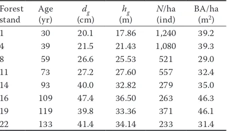
Table 1. Basic characteristics of selected forest stands
Forest
stand Age (yr) (cm)dg (m)hg N(ind)/ha BA/ha (m2)
1 30 20.1 17.86 1,240 39.2
4 39 21.5 21.43 1,080 39.3
8 59 26.6 25.53 521 29.0
11 73 27.2 27.60 557 32.4
14 93 40.0 32.82 279 35.0
16 109 47.4 36.50 263 46.3
19 119 39.8 33.36 371 46.1
22 133 41.4 34.14 233 31.4
tervals were selected, as the second method of cali-bration (only trees in the interval around the mean diameter) was proved unsatisfactory. The reason was that in this case the calibration very often failed because the resulting model had too high values of compared criteria (in the coefficient of determina-tion too small) and the actual model did not meet the conditions required for the correct behaviour of the height function. The most frequent problem was that the fitted heights decreased with increas-ing diameter at breast height. This problem oc-curred in the variant with all numbers of selected trees (1 to 5), so that even the larger sample size did not eliminate this problem. Conversely, calibration with trees in three diameter intervals worked prop-erly at all times.
The results in Table 3 show that the LME model, which uses calibration data measured on trees in three diameter intervals, is reasonable. With the in-creasing number of measured trees, the goodness
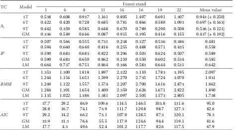
[image:5.595.63.538.420.683.2]of fit of the model grows as well. If a comparison is made of results obtained using the LME model and results of the generalized model, it is evident that the LME model with three measured trees provides sig-nificantly worse results. The mean of deviations of the fitted values is on average (indifferently for forest stands) more than double than that of the general-ized model. Conversely, when comparing the LME model with nine measured trees and the generalized model, better results for R2, RMSE, and AIC were achieved in the LME model. The mean of deviations of the fitted values for the LME model is still higher than that of the generalized model, but only by 10 cm on average. In four stands the LME model achieved even better results than the generalized model. In the light of the results obtained, it can be concluded that the LME model with nine trees measured for the calibration purposes achieves similar results like the generalized model and can therefore be used in place of it. If both types of tested models (the LME Table 3. Criteria of evaluated models
TC Model 1 4 8 11 14Forest stand16 19 22 Mean value
Δi
3T 0.538 0.608 0.937 1.161 0.805 1.497 0.691 1.307 0.943 (± 0.250)
6T 0.422 0.420 0.728 0.685 0.781 0.866 0.580 1.093 0.697 (± 0.163)
9T 0.442 0.359 0.585 0.648 0.670 0.789 0.290 0.508 0.536 (± 0.121)
GM 0.336 0.549 0.646 0.087 0.915 0.395 0.416 0.155 0.437 (± 0.192)
R2
3T 0.507 0.566 0.555 0.731 0.238 0.327 0.536 0.386 0.481
6T 0.594 0.660 0.640 0.816 0.255 0.488 0.571 0.435 0.558
9T 0.590 0.683 0.683 0.822 0.296 0.503 0.624 0.507 0.589
GM 0.590 0.683 0.650 0.862 0.210 0.550 0.602 0.534 0.585
LM 0.664 0.737 0.751 0.864 0.366 0.583 0.644 0.531 0.642
RMSE
3T 1.353 1.300 1.818 1.897 2.322 3.110 1.783 3.195 2.097
6T 1.244 1.154 1.651 1.599 2.270 2.735 1.724 3.070 1.931
9T 1.249 1.122 1.557 1.574 2.207 2.700 1.616 2.873 1.862
GM 1.284 1.301 1.654 1.400 2.359 2.626 1.671 2.822 1.890
LM 1.135 1.022 1.386 1.381 2.097 2.505 1.573 2.805 1.738
AIC
3T 37.7 29.2 86.9 109.6 114.5 146.5 103.8 131.6 95.0
6T 28.8 16.7 74.1 73.9 111.7 129.8 98.7 127.3 82.6
9T 29.2 14.2 66.2 73.1 107.9 128.5 87.3 120.1 78.3
GM 33.9 31.3 76.4 55.5 117.9 124.6 94.4 119.1 81.6
LM 17.7 4.3 49.6 52.4 101.2 117.7 82.6 117.5 67.9
TC – type of criterion, Δi – mean of deviations of fitted values obtained from the LME or generalized model and fitted values obtained from the NLR local model (values in brackets are confidence intervals of the mean), R2 – coefficient of
de-termination, RMSE – root mean square error, AIC – Akaike information criterion, 3T – calibrated LME model based on 3 measured trees, 6T – calibrated LME model based on 6 measured trees, 9T – calibrated LME model based on 9 measured trees, GM – generalized model, LM – local model
Table 2. Results of the linear mixed effects 2nd level model
a0 a1 b0 b1 τa2 τ
b
2 τ
ab σ2
1.2587* (0.18139) 0.6891* (0.05195) –5.3048* (1.29638) –0.1863* (0.04008) 0.0035 1.6595 –0,0012 0.0041
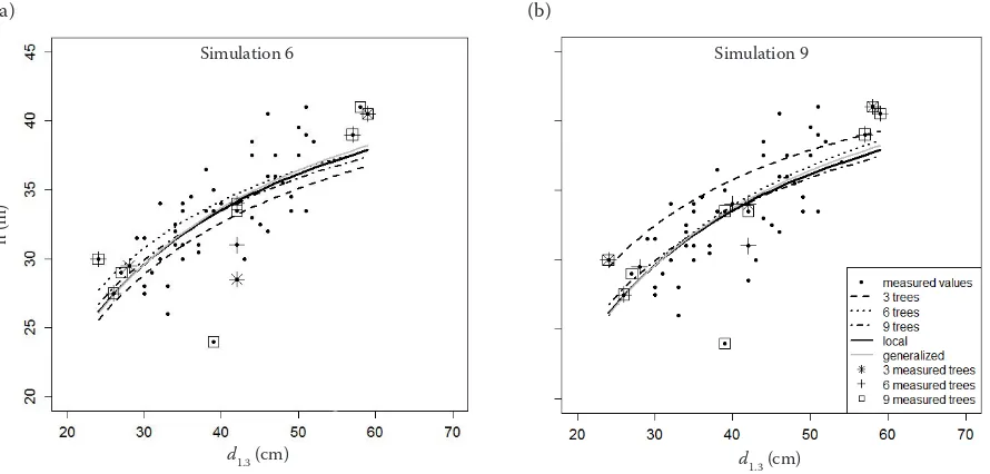
and generalized model) were compared with the local model, it was found that there are differences between models, but in practical terms these differ-ences are acceptable. Both compared types of mod-els can thus be used instead of the local model of the height curve. In the LME model, the above applies only when more trees are used for calibration (6 to 9). The quality of both compared models against the lo-cal model can be well seen in Fig. 1a, which shows all the constructed models by the example of forest stand no. 22.
In the mixed model it is also better to use cali-bration based on a greater number of trees on the grounds that it better describes the variability of heights in individual diameter intervals. This leads to stabilization of the height curve position. For cali-bration based on smaller samples the curve position is more influenced by even one biased value. This means that if dominant, or conversely, suppressed tree is selected for calibration, the curve position is biased towards this individual. Stabilization of the position of the resulting curve, and its resistance to outliers causing bias are seen in Fig. 1b, which shows the influence of the number of measured trees by the example of forest stand no. 22. The position of the curve constructed by the LME model, which was calibrated on the basis of three measured trees, is significantly biased when compared with the lo-cal model. That is because two dominant trees were measured (one with small diameter and one with large diameter). The position of the height curve constructed by the LME model calibrated through measurement of nine trees is no longer biased, al-though the same two trees were also selected.
DISCUSSION
Within the LME model, two types of tree selec-tion for condiselec-tional calibraselec-tion were tested. A mod-el, which is based on selection of trees only in the interval of mean diameter, proved unsuitable be-cause it had poor values of the monitored criteria or was not biologically justified. Crecente-Campo et al. (2010) also tested the conditional calibration with selection of trees within the mean diameter. The difference was only in the fact that they used the nonlinear mixed effects modelling approach to construct the height curve. Their sample size for calibration was 1 to 10 trees. Nor did they describe this method of selection as suitable, because models constructed using this method for calibrating had a very high mean of residuals and standard errors. Also Özcelik et al. (2013) confirmed in their work the high mean of residuals at the same calibration method. But it is arguable that the mean of residuals, standard error of residuals as well as the root mean square error decrease when a larger sample size is used for calibration, regardless of the method of selection (Trincado et al. 2007; Kangas, Haara 2012). This hypothesis was confirmed in this study only partially, and only in the case of selection made from three diameter intervals.
[image:6.595.67.512.56.269.2]Very good results were achieved in the model where the tree selection was made in three diame-ter indiame-tervals. While the variant with a single tree in each diameter interval displayed high values of the mean of deviations of fitted values obtained from the LME model and fitted values obtained from the NLR local model, they decreased when a larger Fig. 1. Forest stand No. 22: (a) comparison of LME (sampled trees from three diameter intervals), generalized and local model; (b) influence of sample size of trees for conditional calibration of LME model
(a) (b)
d1.3 (cm) d1.3 (cm)
h (m)
sample size of trees was chosen within the inter-vals. When selecting three trees in each interval, in the half of the forest stands this mean of devia-tions was even less than in the generalized model. For other monitored criteria better results were achieved with the LME model than with the gen-eralized model in all forest stands. In their work, Crecente-Campo et al. (2010) and Özcelik et al. (2013) used the same methodology for the selection of trees (3, 6 or 9 in three diameter intervals). Both of these studies arrived at the same conclusion that when trees are selected from more diameter inter-vals, the quality of the model is significantly better.
For the generalized model we have determined the mean height hg as a function of dg with using the local model. According to Šmelko (2007) it is one of the standard ways of hg determination. Another standard way is a procedure where a certain num-ber of trees with diameter <dg ± 2 cm> is found, their heights are measured and arithmetic mean is calculated. This is also taken as the mean height hg of the stand. The latter way was not used because there was not a sufficient number of trees with di-ameter <dg ± 2 cm> on sample plots. For first way of hg determination, Van Laar and Akca (2007) recommended 20 to 25 height measurements. For the second way of hg determination, Halaj (1955) recommended to measure 9 to 22 heights for the whole stand depending on its size and to divide this number in direct proportion to the species composition. Šmelko (2007) proposes determin-ing this number accorddetermin-ing to the stand height vari-ability and raising it by several heights compared to Halaj (1955) in order to achieve higher accuracy. Šmelko (2007) indicates that if the mean height hg is determined by measuring 10 to 25 heights in <dg ± 2 cm>, it is possible to determine the mean height with the standard error of ± 2%. It is there-fore apparent that in using the generalized model, we need to measure more heights than in the case of the calibrated LME model. For this reason, the LME model can be classified as an effective meth-od in terms of the time required for measurements (Crecente-Campo et al. 2010; Zhao et al. 2013).
As a generalized model, the model constructed by Šmelko et al. (1987) was chosen. Alternatively, the generalized model by Wolf (1978) can be used. This model is also based on the Michailoff function using mean diameter and mean height. Its perfor-mance is practically identical to the actual model used. Its disadvantage is that it has set the param-eters for spruce only.
The results have shown that according to most criteria the LME model provides better results
than the generalized model. The same results were obtained e.g. by Sharma and Parton (2007), who compared the generalized model and nonlinear mixed effects (NLME) model for more boreal tree species in Ontario as well as Vargas-Larreta et al. (2009), who compared the NLME model and generalized model for different tree species in Du-rango, Mexico.
Our generalized model used mean diameter and mean height as stand variables. Both variables are often used because they describe the stage of stand development. For example, Wolf (1978) used the same stand variables in his generalized model and achieved very similar results in terms of quality of the resulting model. The same variables were used also by Adame et al. (2008), who in addition to these two stand variables tested also dominant height and dominant diameter, stand basal area per hectare and number of trees per hectare. Their model was best when they used stand basal area and dominant height. Good results using the gen-eralized model were also obtained by Schröder and Álvarez-Gonzáles (2001), who used mean diameter, Soares and Tomé (2002), who used dominant height and Temesgen and von Gadow (2004) or Temesgen et al. (2014), who used the stand variables like stand basal area per hectare, number of trees per hectare and stand basal area of larger trees per hectare.
CONCLUSIONS
curve (e.g. the continually increasing function). The advantage of the calibrated LME model against the generalized model is that the model of the same quality is achieved when measuring a smaller number of heights. In this case, we have measured maximally 9 heights in the LME model. In the generalized model, it is recommended that 10 to 25 heights are measured. This number is directly and proportionally dependent on the variability of heights within the forest stand. The LME model is thus able to achieve the same (or better) results than the generalized model, but at a lower intensity of measurements in terms of both time and money.
Acknowledgements
The author would like to thank Karel Drápela and Jan Kadavý for their valuable comments and two anonymous reviewers for numerous notes that helped him improve the article quality.
References
Adame P., Del Río M., Cañellas I. (2008): A mixed nonlinear height-diameter model for pyrenean oak (Quercus pyrena-ica Willd.). Forest Ecology and Management, 256: 88–98. Adamec Z., Drápela K. (2015): Generalized additive models as an alternative approach for the modelling of the tree height-diameter relationship. Journal of Forest Science, 61: 235–243.
Akaike H. (1973): Information theory and an extension of the maximum likelihood principle. In: Petrov B.N., Csaki F. (eds): Proceedings of the 2nd International symposium
on information theory, Budapest, Sept 2–8, 1973: 268–281. Calama R., Montero M. (2004): Interregional nonlinear
height-diameter model with random coefficients for stone pine in Spain. Canadian Journal of Forest Research, 34: 150–163.
Calama R., Montero G. (2005): Multilevel linear mixed model for tree diameter increment in stone pine (Pinus pinea): a calibrating approach. Silva Fennica, 39: 37–54.
Castedo-Dorado F., Barrio-Anta M., Parresol B.R., Álvarez-González J.G. (2005): A stochastic height-diameter model for maritime pine ecoregions in Galicia (northwestern Spain). Annals of Forest Science, 62: 455–465.
Crecente-Campo F., Tomé M., Soares P., Diéguez-Aranda U. (2010): A generalized nonlinear mixed-effects height-diameter model for Eucalyptus globulus L. in northwestern Spain. Forest Ecology and Management, 259: 943–952. Curtis R.O. (1967): Height-diameter and height-diameter-age
equations for second-growth douglas-fir. Forest Science, 13: 365–375.
Drápela K. (2011): Regresní modely a možnosti jejich využití v lesnictví. [Habilitation Thesis.] Brno, Mendel University in Brno: 235.
Eerikäinen K. (2003): Predicting the height-diameter pattern of planted Pinus kesiya stands in Zambia and Zimbabwe. Forest Ecology and Management, 175: 355–366.
Fabrika M., Pretzsch H. (2013): Forest Ecosystem Analysis and Modelling. Zvolen, Technická univerzita vo Zvolene: 620. Fang Z., Bailey R.L. (1998): Height-diameter models for
tropical forest on Hainan Islands in Southern China. Forest Ecology and Management, 110: 315–327.
Halaj J. (1955): Tabuľky na určovanie hmoty a prírastku porastov. Bratislava, SVPL: 328.
Huang S., Price D., Titus S.J. (2000): Development of ecoregion-based height-diameter models for white spruce in boreal forests. Forest Ecology and Management, 129: 125–141.
Huang S., Titus S.J., Wiens D.D. (1992): Comparison of non-linear mixed height-diameter function for major Alberta tree species. Canadian Journal of Forest Research, 22: 1297–1304.
Husch B., Beers T.W., Kershaw J. A. (2003): Forest Mensura-tion. 4th Ed. Hoboken, New Jersey, John Wiley & Sons: 443.
Kangas A., Haara A. (2012): Comparison of nonspatial and spatial approaches with parametric and nonparametric methods in prediction of tree height. European Journal of Forest Research, 131: 1771–1782.
Lu J., Zhang L. (2013): Evaluation of structure specification in linear mixed models for modeling the spatial effects in tree height-diameter relationships. Annals of Forest Research, 56: 137–148.
Martin F., Flewelling J. (1998): Evaluation of tree height prediction models for stand inventory. Western Journal of Applied Forestry, 13: 109–119.
Mehtätalo L. (2004): A longitudinal height-diameter model for Norway spruce in Finland. Canadian Journal of Forest Research, 34: 131–140.
Michailoff I. (1943): Zahlenmäßiges Verfahren für die Ausfüh-rung der Bestandeshöhenkurven. Forstwissenschaftliches Centralblatt und Tharandter Forstliches Jahrbuch, 6: 273–279. Özçelik R., Diamantopoulou M.J., Crecente-Campo F., Eler
U. (2013): Estimating Crimerian juniper tree height using nonlinear regression and artificial neural network models. Forest Ecology and Management, 306: 52–60.
Petterson H. (1955): Barrskogens volymproduktion. Med-delanden från Statens skogsforskningsinstitut, 45: 1–391. Prodan M. (1951): Messung der Waldbestände. Frankfurt a.
M., J.D. Sauerländer's Verlag: 260.
R Development Core Team (2015): R: A language and en-vironment for statistical computing. R Foundation for Statistical Computing, Vienna, Austria. Available at http:// www.R-project.org/ (accessed March 1, 2015).
Schmidt M., Kiviste A., von Gadow K. (2011): A spatially explicit height-diameter model for Scots pine in Estonia. European Journal of Forest Research, 130: 303–315. Schröder J., Álvarez-Gonzáles J.G. (2001): Comparing the
performance of generalized diameter-height equations for maritime pine in Northwestern Spain. Forstwissenschaftli-ches Centralblatt, 120: 18–23.
Sharma M., Parton J. (2007): Height-diameter equations for boreal tree species in Ontario using a mixed-effects modeling approach. Forest Ecology and Management, 249: 187–198.
Sharma M., Zhang S.Y. (2004): Height-diameter models using stand characteristics for Pinus banksiana and Picea mari-ana. Scandinavian Journal of Forest Research, 19: 442–451. Soares P., Tomé M. (2002): Height-diameter equation for first
rotation eucalypt plantations in Portugal. Forest Ecology and Management, 166: 99–109.
Šmelko Š. (2007): Dendrometria. Zvolen, Technická univer-zita vo Zvolene: 400.
Šmelko Š., Pánek F., Zanvit B. (1987): Matematická formulácia systému jednotných výškových kriviek rovnovekých poras-tov SSR. Acta Facultatis Forestalis Zvolen, 19: 151–174. Temesgen H., von Gadow K. (2004): Generalized
height-diameter models – an application for major tree species in complex stands of interior British Columbia. European Journal of Forest Research, 123: 45–51.
Temesgen H., Zhang C.H., Zhao X.H. (2014): Modelling tree height-diameter relationships in species and multi-layered forests: A large observational study from Northeast China. Forest Ecology and Management, 316: 78–89. Trincado G., VanderSchaaf C.L., Burkhart H.E. (2007):
Re-gional mixed-effects height-diameter models for loblolly pine (Pinus taeda L.) plantations. European Journal of Forest Research, 126: 253–262.
Van Laar A., Akça A. (2007): Forest Mensuration. Managing Forest Ecosystems. Volume 13. Dordrecht, Springer: 383. Vargas-Larreta B., Castedo-Dorado F., Alvarez-Gonzalez
F.J., Barrio-Anta M., Cruz-Cobos F. (2009): A general-ized height-diameter model with random coefficients for uneven-aged stands in El Salto, Durango (Mexico). Forestry, 82: 445–462.
Vonesh E.F., Chiinchilli V.M. (1997): Linear and nonlinear models for the analysis of repeated measurements. Boca Raton, Chapman & Hall/CRC: 560.
Wolf J. (1978): Systém standardizovaných výškových křivek stejnověkých smrkových porostů. Acta Universtitatis Agri-culturae Brno. Series C, Facultas silviAgri-culturae, 47: 93–102. Yang Y., Huang S. (2011): Comparison of different methods
for fitting nonlinear mixed forest models and for making predictions. Canadian Journal of Forest Research, 41: 1671–1686.
Zhang L. (1997): Cross-validation of non-linear growth function for modelling tree height-diameter relationships. Annals of Botany, 79: 251–257.
Zhang L., Bi H., Cheng P., Davis C.J. (2004): Modeling spatial variation in tree diameter-height relationships. Forest Ecol-ogy and Management, 189: 317–329.
Zhang L., Ma Z., Guo L. (2008): Spatially assessing model er-rors of four regression techniques for three types of forest stands. Forestry, 81: 209–225.
Zhao L., Chunming L., Tang S. (2013): Individual-tree diam-eter growth model for fir plantations based on multi-level linear mixed effects models across southeast China. Journal of Forest Research, 18: 305–315.
Received for publication July 7, 2015 Accepted after corrections October 12, 2015
Corresponding author: